Sensible Gamblers’ Guide to Shorting Volatility

Everything you need to know about variance risk premium

The first time I learned about the concept of short volatility was when James Cordier posted a now-legendary apology video to YouTube after blowing his fund..

Shortly after the video started getting traction online, I got curious how he actually blew up and learned that he managed to do so by selling naked options on natural gas and crude oil.

This theme of massive blowouts of short vol strategies kept repeating over and over throughout the history but also during COVID, which came shortly after.

So why do people do it? Why, if you search “options strategies” on YouTube, are there thousands of videos promoting “selling options for income”?

I would like to explore that in today’s article, but not only that.

Throughout the years I have developed a short volatility strategy that consistently works. Considering the fact I still have a roof over my head after many of the recent market stresses, I decided to share it step by step with all the rules, data, and backtests.

All the data you will see in this article comes from tradingriot.com. There you can find all relevant charts, screeners, and calculators, which allow you to start trading this strategy yourself.

Why selling volatility makes money

If you are coming from the simpler side of trading space and you spend your days drawing lines on charts and convincing yourself that the twenty-something-year-old trader you are watching on YouTube really made his money by trading 1-minute charts of Nasdaq futures for 15 minutes a day. You might have no idea what I am actually talking about.

I don’t want this article to be a 101 explainer on options. I have a whole course about trading basics on my website, which is completely free, so make sure you read that if you have some gaps in options trading.

In short, trading futures gives traders linear types of payoff structure: if you have a long future and the market goes up, you make money; if it goes down, you will lose money.

Things are slightly more complicated with options; when you buy or sell an option, the change in the underlying asset is only one part of the equation.

Besides that, time, volatility, and interest rates (no one cares about those) play a role as well.

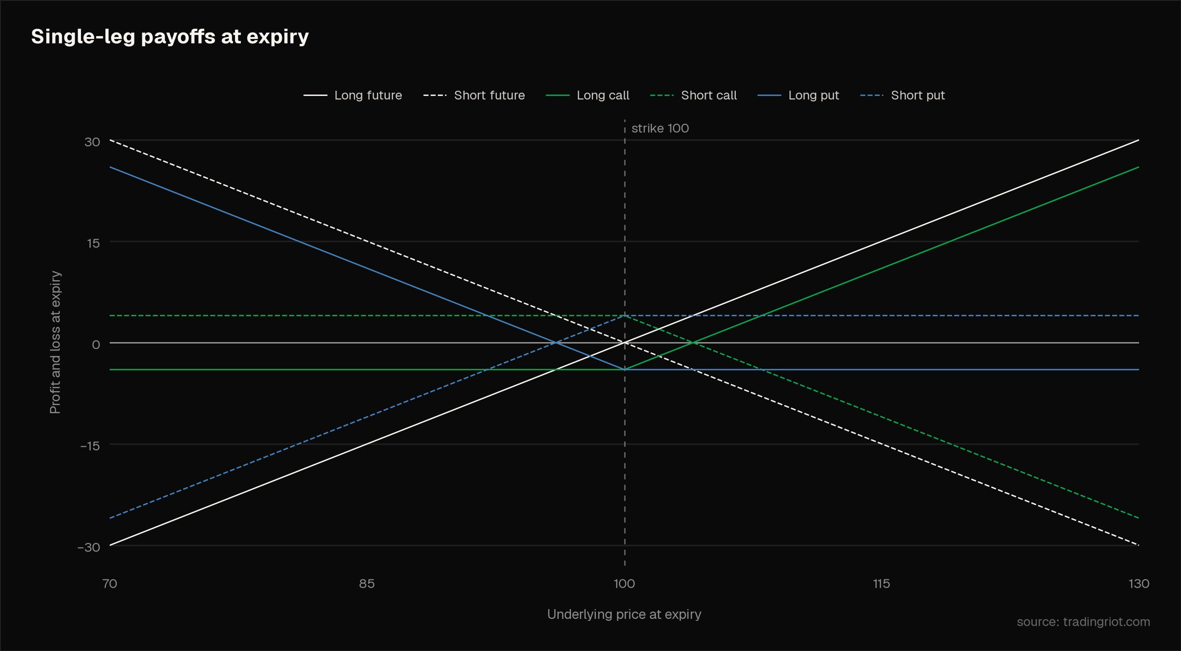
This volatility component is what matters here, as with options you create positions that make or lose money based on markets’ realized volatility, no matter the move in the underlying asset.

Volatility

When we are looking at volatility for each market, you often see two different names, implied and realized volatility.

Realized volatility is pretty simple; it is the annualized standard deviation of the returns of underlying assets over some past window.

I don’t want you to confuse you too much, but there are a bunch of different models and calculations so the realized volatility number you see in different platforms can differ even on the same look back.

One of the simpler measures and the one I also use is close-to-close realized volatility.

You take a series of daily closing prices, compute daily log returns, compute the standard deviation of those returns over your chosen window, and annualize by multiplying by the square root of 252 (trading days per year; for crypto options, use 365):

sigma_annual = sigma_daily x sqrt(252)

If you are considering closing this article now, here is a much simpler explainer:

You figure out how big a typical daily wiggle has been, then scale it up to a yearly number so it will match the implied volatility quotes since those are always annualized.

The square root is doing the scaling because variances add across independent periods while standard deviations do not. Uncertainty over a whole year works out to roughly 16 times the daily uncertainty, since sqrt(252) is 15.87 and 16 is close enough.

This 16 number is good to remember since your square root of 252 is 15.87, which is close enough to 16.

When you see a stock with 20-day realized volatility of 32, you can divide 32 by 16; the typical daily move over those last 20 days is 2%. To be more precise, “typical” is actually the daily standard deviation. If daily returns were normally distributed, roughly two thirds (68%) would close within 2%.

The shorter look-back windows, such as 20 days, will be more affected by shorter-term wiggles, while the larger look-back windows will be more smoothed but can also react late to market changes. For this article and strategy that follows, we will use the realized volatility lookback, which matches the implied volatility of the option.

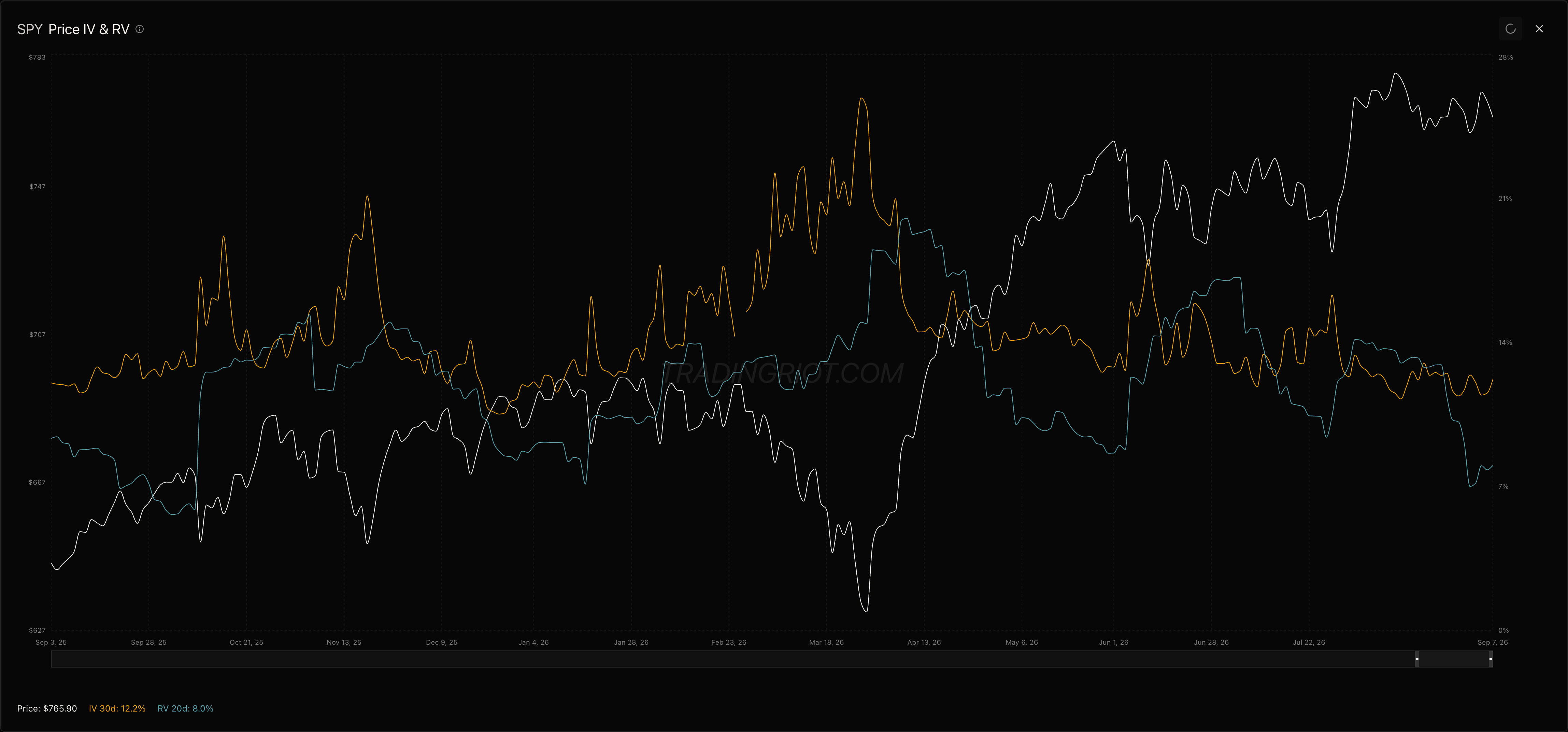
This number does not only include the future price movement; it also includes risk compensation, hedging costs, and supply and demand.

While the realized volatility is backward-looking, implied volatility is different; it tells us what the market thinks future volatility will be. Implied volatility is a forecast over the life of the option, so a 30-day IV is a statement about the next 30 days.

When you are selling volatility, the premium you actually collected is today’s implied against the volatility realized over the following 30 days; assuming you do not have a crystal ball, you will only know once those 30 days are gone. But this doesn’t make realized volatility useless. The trailing comparison tells you whether options look rich right now relative to how the market has been behaving, which is a reasonable starting point.

Implied volatility carries more than a forecast of future price movement. It also carries risk compensation, hedging costs, and plain supply and demand, all of which push the quoted number above what tends to get realized. That persistent gap between what options price in and what the market delivers is called the variance risk premium.

Variance risk premium

Variance risk premium (also called volatility risk premium, which is actually more correct since variance premium is defined on squared terms) is one of the most documented phenomena in options markets.

This is why I am also sharing this whole strategy and concept with you. There is no alpha here, as this is something that has been documented over decades and is very unlikely to go away despite more people trading it.

Variance risk premium describes the tendency of implied volatility to sit above the volatility that ends up being realized.

Variance risk premium in SPX

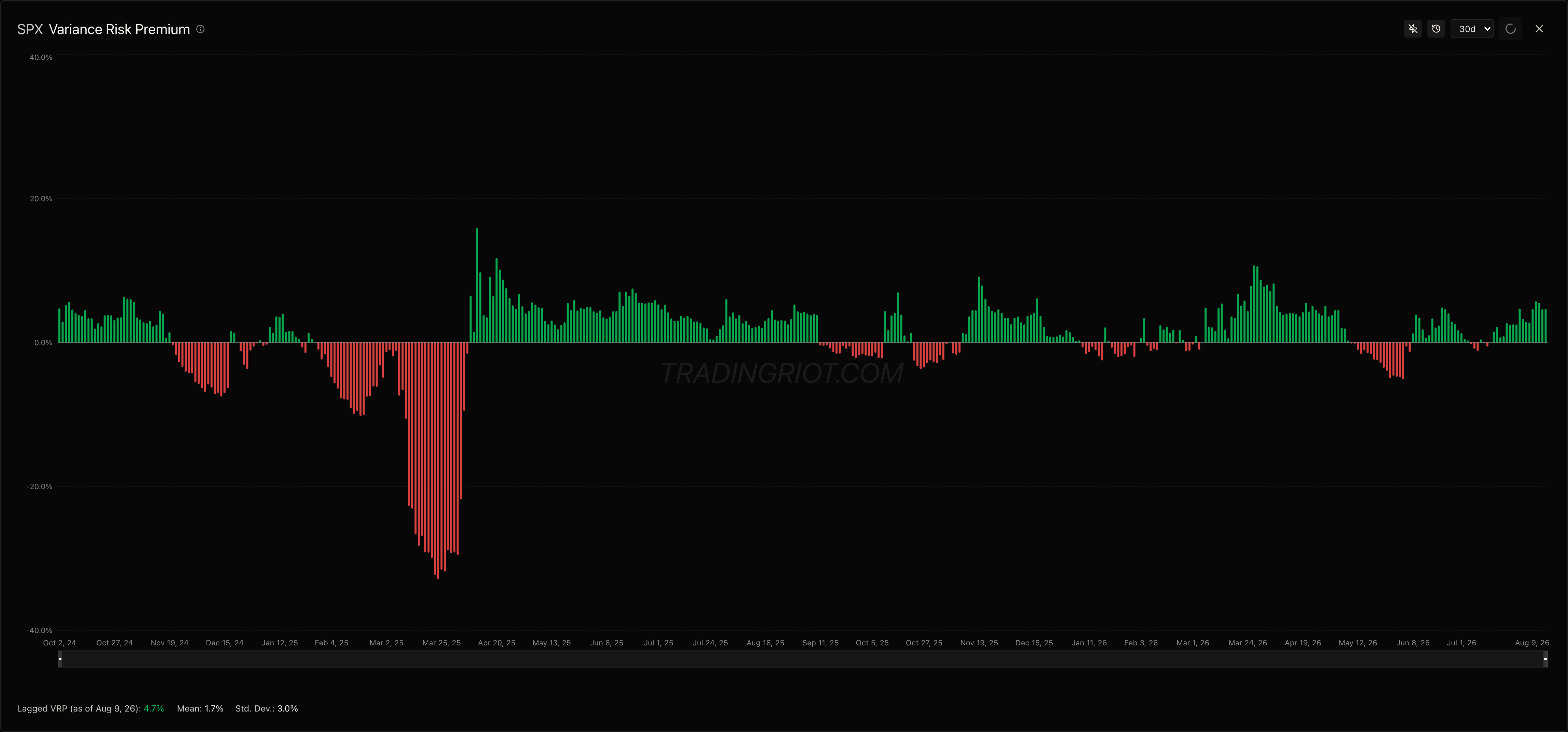
This does not necessarily mean that all options are overpriced, this is the common fallacy of the selling options for the income crowd which might be topic for some other times.

But what VRP does create is a structural edge that can be a consistent source of profits if harvested properly.

The concept of insurance companies is often used when talking about options selling strategies. We will come back to this when we are talking about the payoff distribution. Besides insurance companies being known to collect small payoffs and face large losses occasionally, they are also very selective when selecting those whom they will insure.

If you are dying, scrambling for your last breath, I guess it will be pretty tough to get good health insurance. Similar to if you live in a wildfire epicenter, insuring your house might be either impossible or costly.

So while options have a tendency to be overpriced, we need to be very selective about which options to sell, as losses are typically much higher than possible gains.

The volatility risk premium is not mispricing waiting to be corrected; it is a risk transfer paid for the same reason insurance premiums exceed actuarially expected losses

Nobody looks at profitable insurance companies and concludes the market for insurance is broken.

Going back to markets and trading, there are several reasons why implied volatility is often higher than realized.

Large numbers of investors overpay for protection and are frequently willing to overpay for it. Out of the money put in, indices are prime examples. If you look at the options chain, you will be able to see that out-of-the-money put options in SPY have much higher IV than calls on the opposite side of the chain. This concept of shadow delta, we will revisit later on.

On the opposite side of this insurance-like behavior are your favorite WallStreetBets heroes buying lotto-like OTM calls and puts for speculation, as these offer huge convex payoffs and require low margin.

We have only spoken about the option buyers so far, but one of the reasons this premium exists also sits with option sellers. If you’ve ever sold options, you know you take the risk of large losses, so obviously you want to get paid for it.

As we also learned at the beginning of the article about James Cordier, the market periodically sends vol sellers into lower tax brackets year after year. During calm stretches, sellers pile in premium compresses and short vol products for retail, making selling vol sound like free money right before a massive spike. After yet another traumatizing event, sellers come back and require more premium for crash risk.

This also makes selling options hard, because the premium over the window, which consists of no disaster, is very difficult to measure. Think about 2019: how nice and easy a time you had before someone decided to eat a bat one day in China.

Overall there is an imbalance in options markets; buying options has fixed risk, requires only the premium to be paid, and is accessible to many traders. Selling options, on the other hand, needs you to put out a large amount of margin so you are well capitalized for any tail moves.

This supply and demand imbalance is also what drives option implied volatilities higher.

So selling volatility is not a free lunch, and for us to be profitable, we need to create a systematic approach while consistently monitoring the associated risks.

Variance risk premium in different assets

Because options are widely available across many markets, a good starting point is deciding what we are actually going to trade.

I mentioned that options tend to price volatility above what the market ends up delivering. That is something you can measure directly by looking at the IV/RV ratio over time.

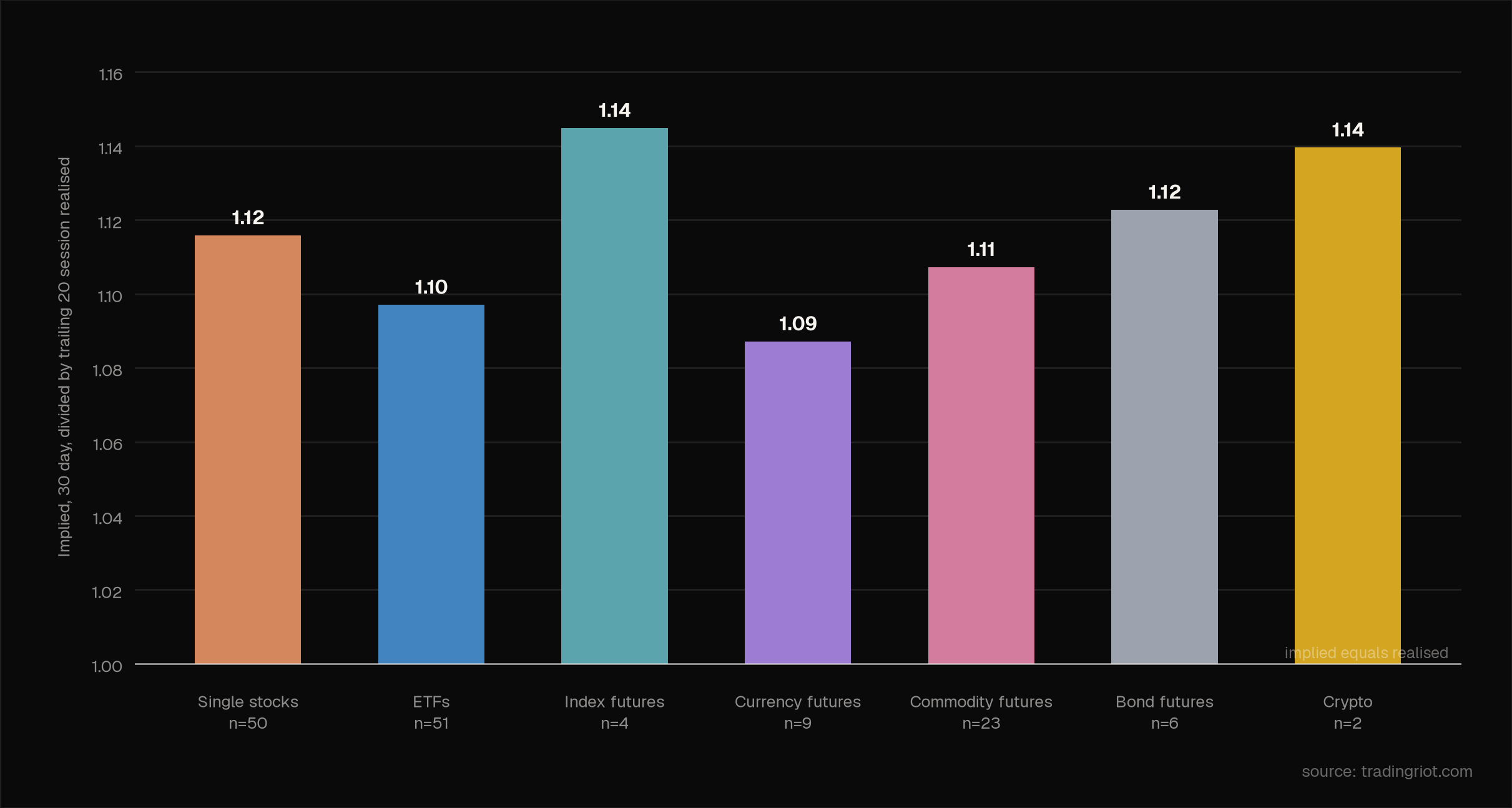
Using data from 2018 on single stocks, ETFs, CME and ICE futures, and crypto, the ratio sits above 1 in every one of them.

As I mentioned before, realized volatility is backward-looking. So knowing that IV sits above RV is useful, but to actually make money, we need the market to realize less than implied over the period ahead.

That is something we can test too, by taking implied volatility against the realized volatility over the next 20 sessions.

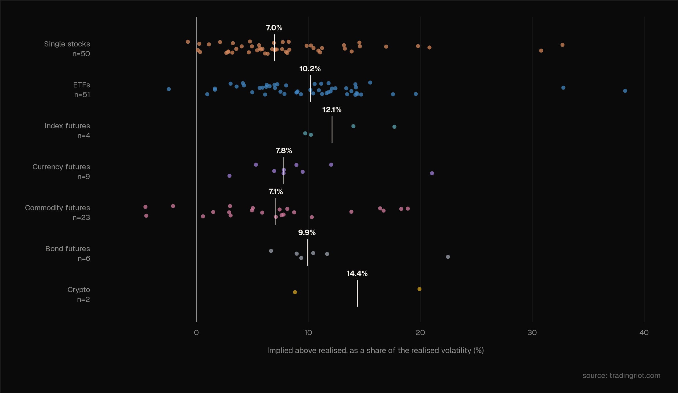
While options on futures markets and ETFs are not the same, they cover the same underlying. ETFs are often cheaper to trade and offer deep liquidity, and you are removing some additional headaches like different contract sizes, roll mechanics, and so on. ETFs also cover crypto these days when documented VRP is rich over time.

This is why the choice can boil down to single-name stocks and ETFs.

Single stocks are tradeable, and I sell volatility on them regularly, but they carry much higher idiosyncratic risk from earnings, company-specific events, and random news.

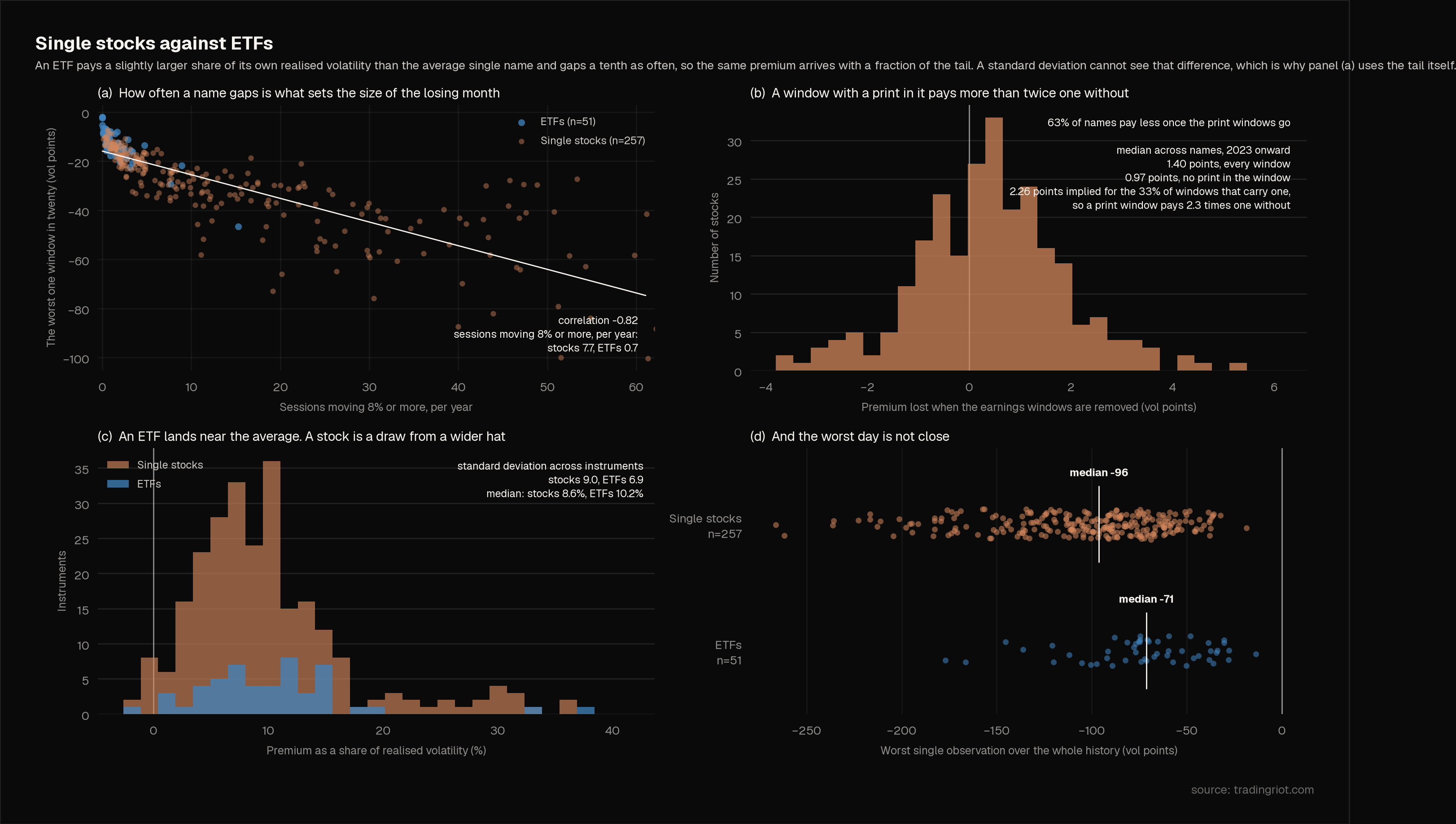
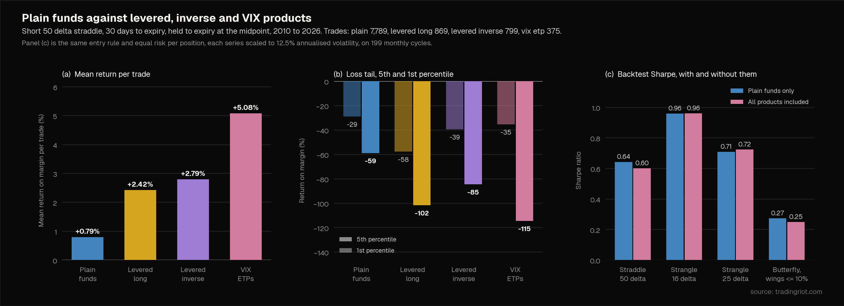
You can clearly see this on the chart above; stocks are moving more on average and gapping more on average, which is opposite of what we want. This is why I am also excluding these going forward; the premium is there, but similar to single-name stocks, they carry a massive tail, and they didn’t have an impactful improvement on the final backtest, which will be shared towards the end of the article.

Stocks with earnings pay more, which makes earnings a tradable event, but it is better to trade earnings volatility in isolation; this might be a topic for another article.

What is the most important here and why we should mostly focus on ETFs is that stocks have much higher tails compared to ETFs.

Options structures and days to expiration

We have established by now that we want to sell volatility and to do it on ETFs.

Now we need to figure out what structures we are going to trade and how many days to expiration they will have.

If you are short options, you are short vega, short gamma, and long theta. You want the market not to move, volatility not to increase, and profits to arrive as time passes.

Gamma sensitivity is highest around the expiration; because of that, selling options with very short days to expiration can be quite tricky.

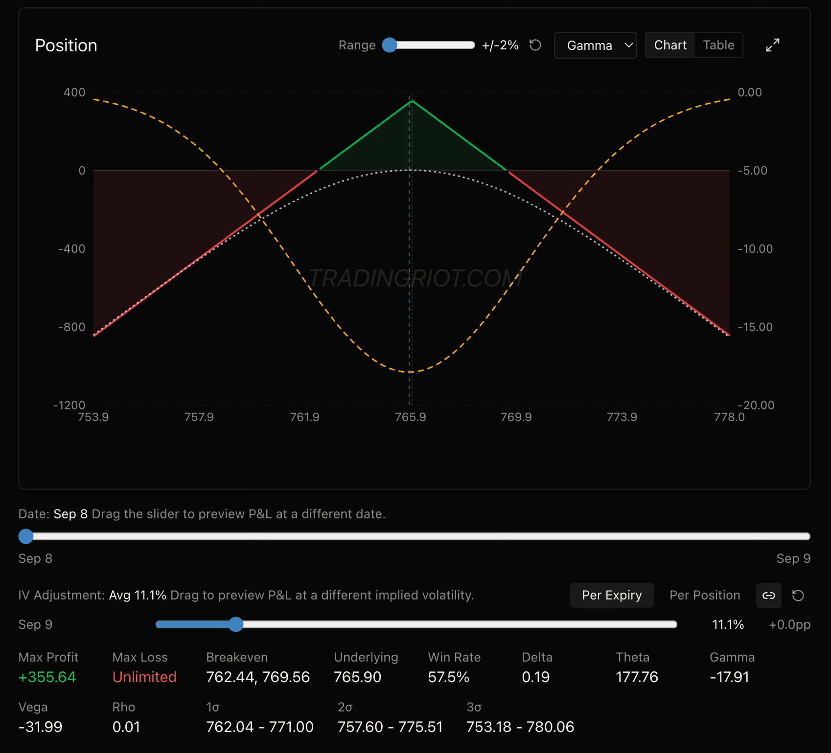
Above is a straddle on SPY expiring tomorrow. The market needs to stay inside about a half percent range for you to make money. Gamma, which is the rate of change in delta, is high here, so a one percent move already puts you outside the profit zone.

You can trade one-day options. What you cannot do is leave your desk while the position is open, and you will not be able to manage many of them at once. This hurts because diversification and the law of large numbers drive a lot of the returns in this business.

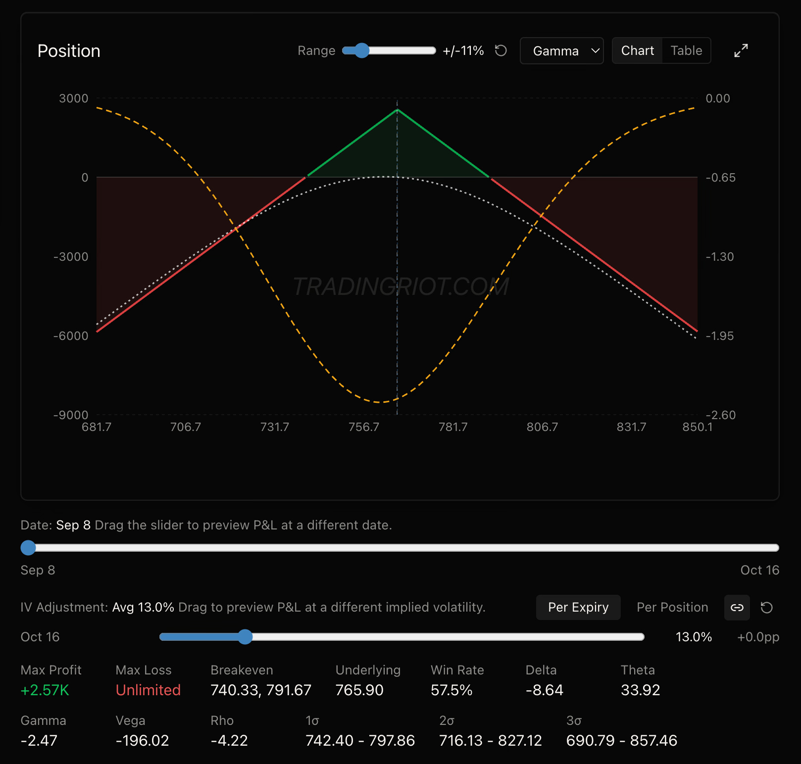
Options expiring in about 40 days from now look much more sensible; you are collecting about seven times the premium, and compared to the change in the underlying, it is more sensitive to what we are actually trading, which is vega—the change in implied volatility.

30- to 60-day options are the sweet spot for this as they have a meaningful decay without extreme gamma from day one. There is enough credit worth your time, and using monthly cycles lets you target the most liquid options.

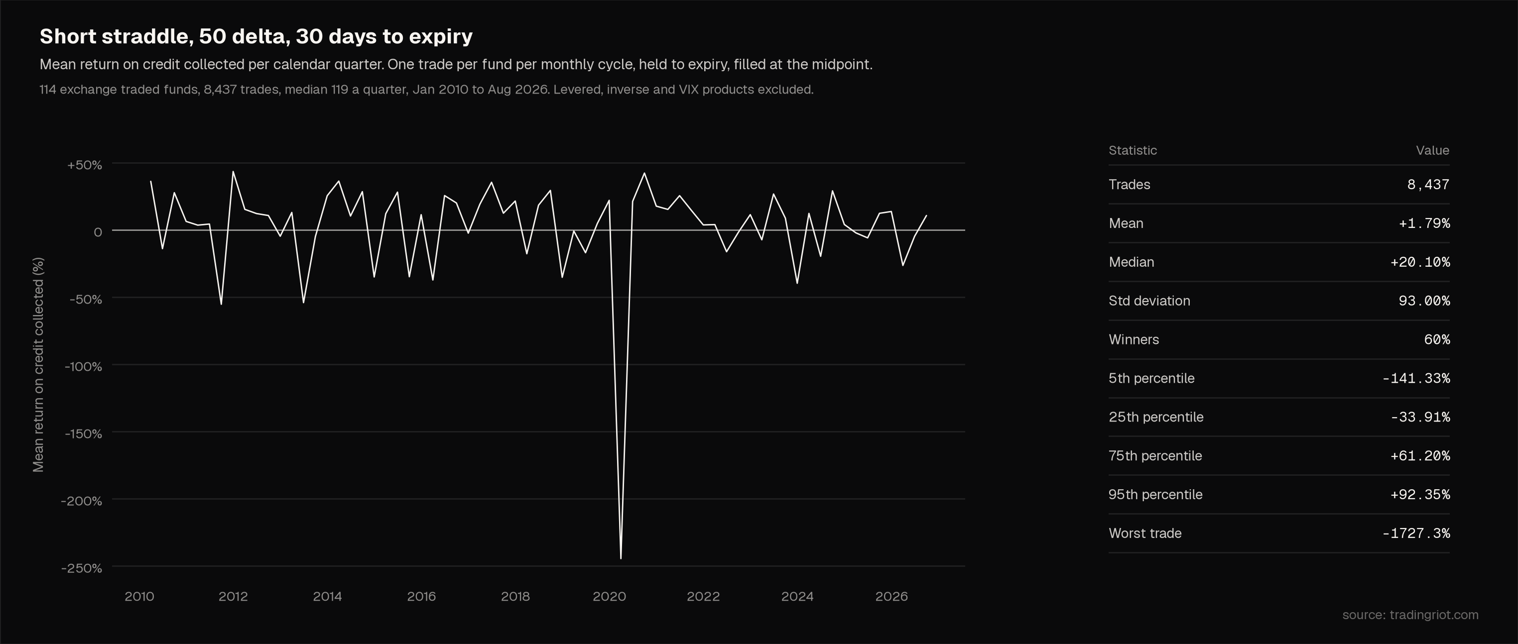
The structure you see on screenshots above is a straddle. You are selling a call and a put at the same strike at the money, nearest to 50 delta. This way, you are going to collect the most premium that is available on the chain since that always sits in the at-the-money options.

Another structure you can go with is a strangle; the idea is the same, but you are selling a call and a put that are out of the money.

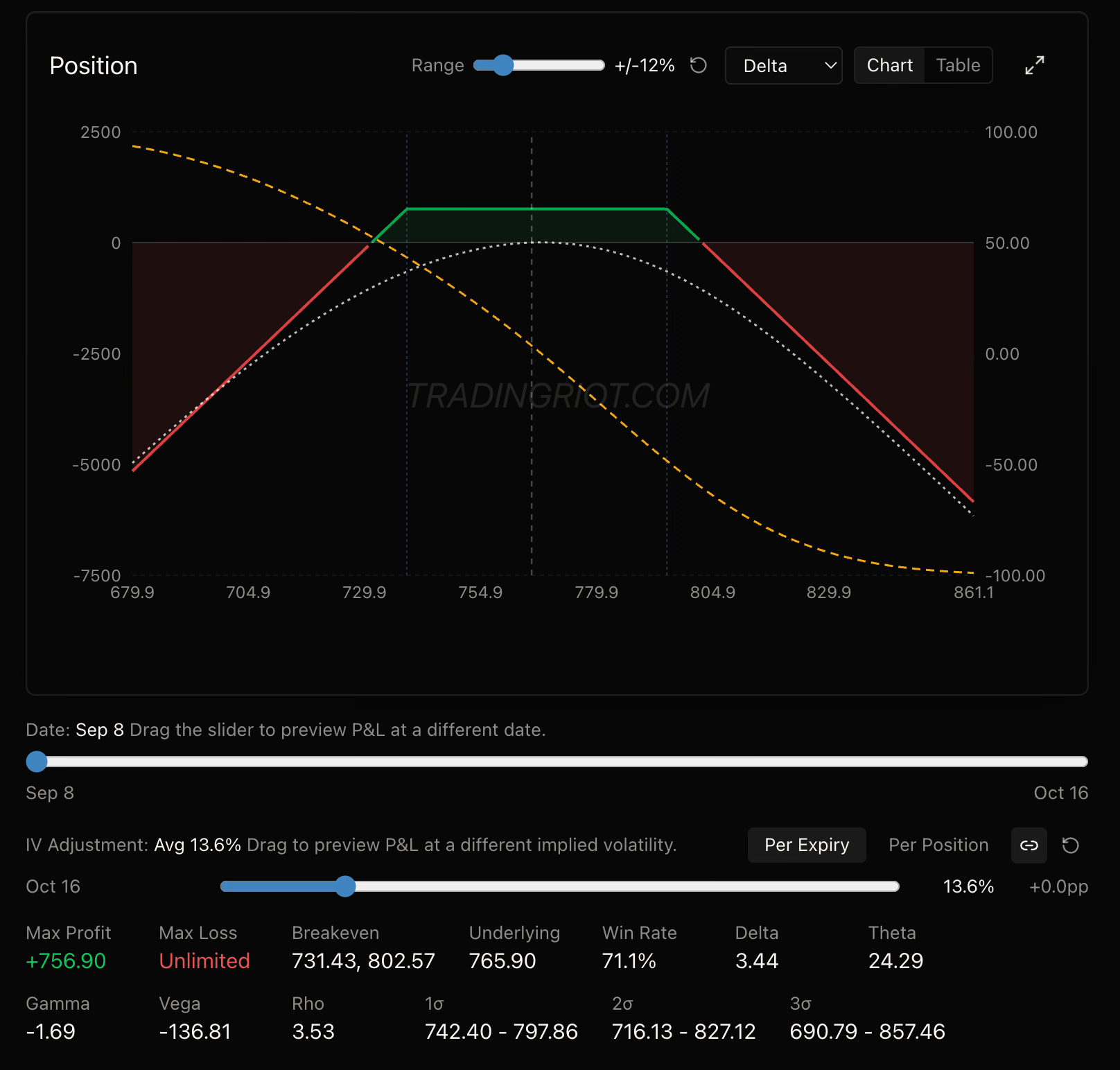
The max profit is much lower compared to a straddle. In exchange, your max profit area is much wider compared to a straddle, where you collect the max profit only if the straddle expires at the strike you originally sold.

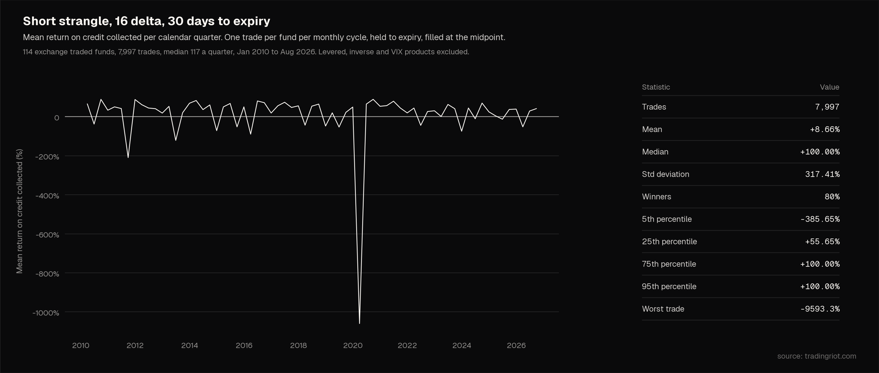
Same as with the straddle chart above, I have run historical returns on a 16 delta strangle. Why 16 delta? Because it is representing roughly a one-standard-deviation move.

If the option market is pricing 20% annualized volatility over the next 30 days, the expected move is around 5.7%, so a 16 delta sits around there on both sides; therefore, you are selling strikes on what the market is pricing.

The second reason for choosing wings around a 15-25 delta is that the vega profile is close to the variance swap.

A variance swap pays the difference between realized variance and a fixed strike without any opinion on direction, and its exposure to volatility stays the same size wherever the underlying happens to be trading.

Straddle does not have it, as it all vega is sitting in one strike, which means that the more drift in the underlying, the less volatility exposure you have. Using strangles, you have roughly the same volatility exposure across the range the underlying is going to visit within the one-sigma move.

While you can’t really trade the variance swaps since they are over-the-counter instruments between dealers and institutions, they are the cleanest expression of the trade this article is about.

Pure exposure to realized against implied with direction stripped out entirely. They are a useful benchmark for what you are trying to approximate with listed options. A 16 delta strangle is pretty close to that.

While this is all nice, if you looked properly on historical returns of both straddle and strangle, you can see that while mean returns are positive, so selling these consistently is a profitable endeavor, they both have fat tails.

No matter how much smart talk and analysis you could have made around these, the COVID crash would find you lying in a fetal position. If you simply sold these structures because implied volatility is over-realized.

Luckily, we can increase our odds of not blowing out.

Increasing the odds

Now we know that selling straddles and strangles works and also sucks.

This is a good thing; the core principle of risk premium strategies is that you are taking a risk others are trying to avoid. That’s where your compensation comes from.

Not everyone wants to be short volatility, facing losses that are magnitudes higher.

That being said, you also shouldn’t strive to be a masochist; I like to sleep at night knowing that if broad markets don’t have five limit-down sessions in a row, I won’t have to send my resume to McDonald’s next week.

Hence, we can try to come up with conditions where we will be selling volatility and conditions where we are going to stay away.

In case you forgot, the core principle is that you want the market to stay calm during the lifetime of your option, so our goal is actually simple; we just need to be able to predict the future—I’m joking, at least partly. We don’t need to predict the future, but we should take a look at filters that will give us a better idea of what subsequent realized volatility will be.

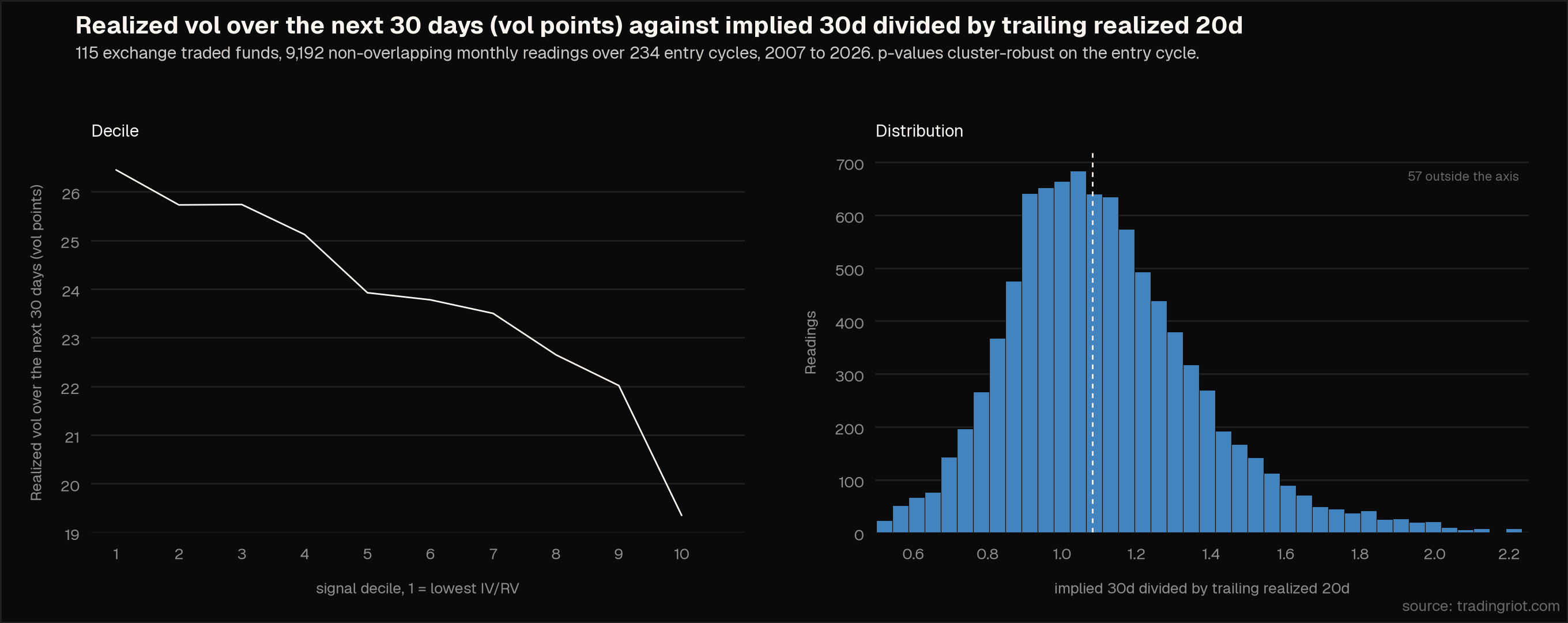
Starting off with what it is: the core of volatility risk premia, which is implied volatility divided by realized.

What we find out in the next several tests is how much markets are going to wiggle over the next month.

When implied volatility is significantly higher than realized, markets are expecting outsized moves, and as you can see, the higher the ratio, the lower the actual realized move ends up being.

This can come back to reasons why this premium exists in the first place, but more importantly, what this test tells us is that the higher the ratio is, the better the potential returns are. Since markets are going to see fewer movements.

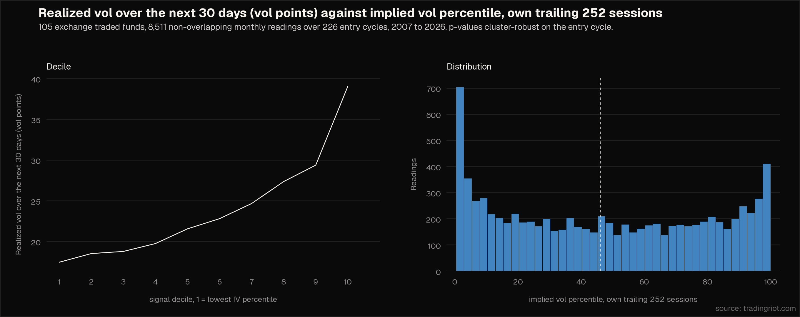
You might think now that all you have to do is to sell volatility when the implied is rich compared to realized, but that’s not exactly the case.

A lot of education about selling options promotes that selling volatility is best when the volatility is high; the IV percentile and rank are often used as indicators.

The chart above shows IV percentile, which is a trailing one-year lookback that spits out a percentage number, so IV percentile at 80% means that IV is higher than 80% of the prior 252 days.

As it turns out, the conventional wisdom is not really correct (shocking, right?); the higher the percentile, the more volatility ends up being realized over the next thirty days, which is not what we are looking for.

In general, the lower the IV percentile, the better it is to sell options. From the chart, you can see that the acceleration really starts after about the seventh decile.

On the other hand, we want to sell options that are rich, as the premiums are more attractive; hence, I only skip those that are above the eighth decile and will use that number going forward.

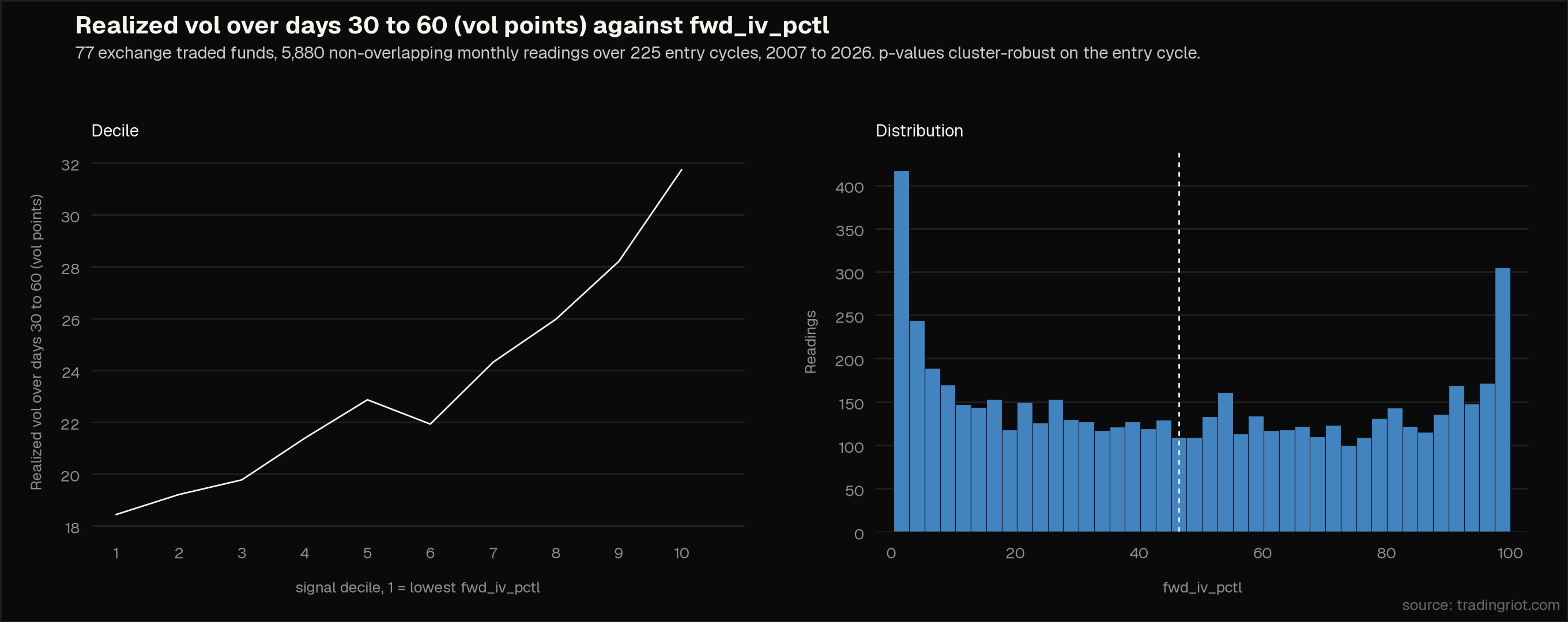
The last one is slightly more complicated, so bear with me. Different days to expiration have different implied volatilities (even different strikes have different implied volatilities, but more on that later).

A thirty-day option is pricing the thirty-day volatility, and a sixty-day option is pricing the sixty-day volatility (duh), but the sixty-day volatility is not a separate forecast; it contains the first one.

This is what forward volatility is all about; in this case it is what the market is pricing for days thirty to sixty.

If the thirty-day implied is 18 and the sixty-day implied is 20, the market is not saying that the second month has implied volatility of 20; it is saying that the whole months are going to average 20, but the first one only 18, so the second month must be doing some extra work.

You might be thinking why this is actually relevant; if we are selling an option that expires in thirty days, all that matters is that markets will be calm for that period and what happens after is not our problem.

Well, that’s not really the case, and it is because one of the main characteristics of volatility is that it clusters. If the market is pricing the shaky next month, it’s usually already quite shaky right now, and the front-month premium we are collecting might not have just caught up yet.

If you are interested in how this is actually calculated, I will be very brief here since I have another strategy which is solely dedicated to trading forward volatility, so to keep things brief, you can’t just add up two volatilities.

But you can add up variance since variance adds up over time and variance is volatility squared multiplied by the time it cover.

Therefore, the 30-60 forward volatility is calculated:

IV60² × 60 = IV30² × 30 + forward² × 30

Divide through by 30 and rearrange:

forward = √( 2 × IV60² − IV30² )

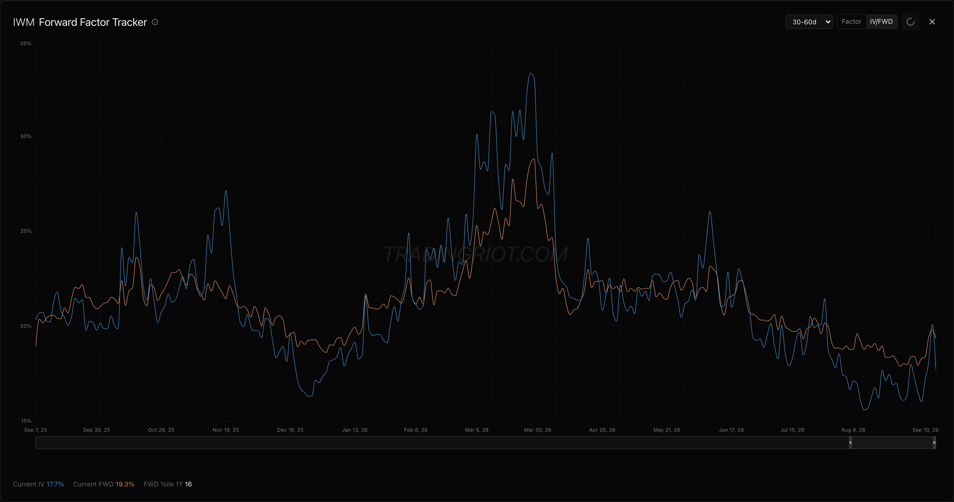
Calculating this number for all ETFs and turning it again into a percentile, we can see that the lower the percentile is, the lower subsequent volatility is realized.

To put simply, if markets are pricing calmer markets between two expirations, we are likely to see lower realized volatility during the lifespan of our option trade.

Do the filters work?

Now that we have established some rules, we need to make sure that they are doing the work wanted.

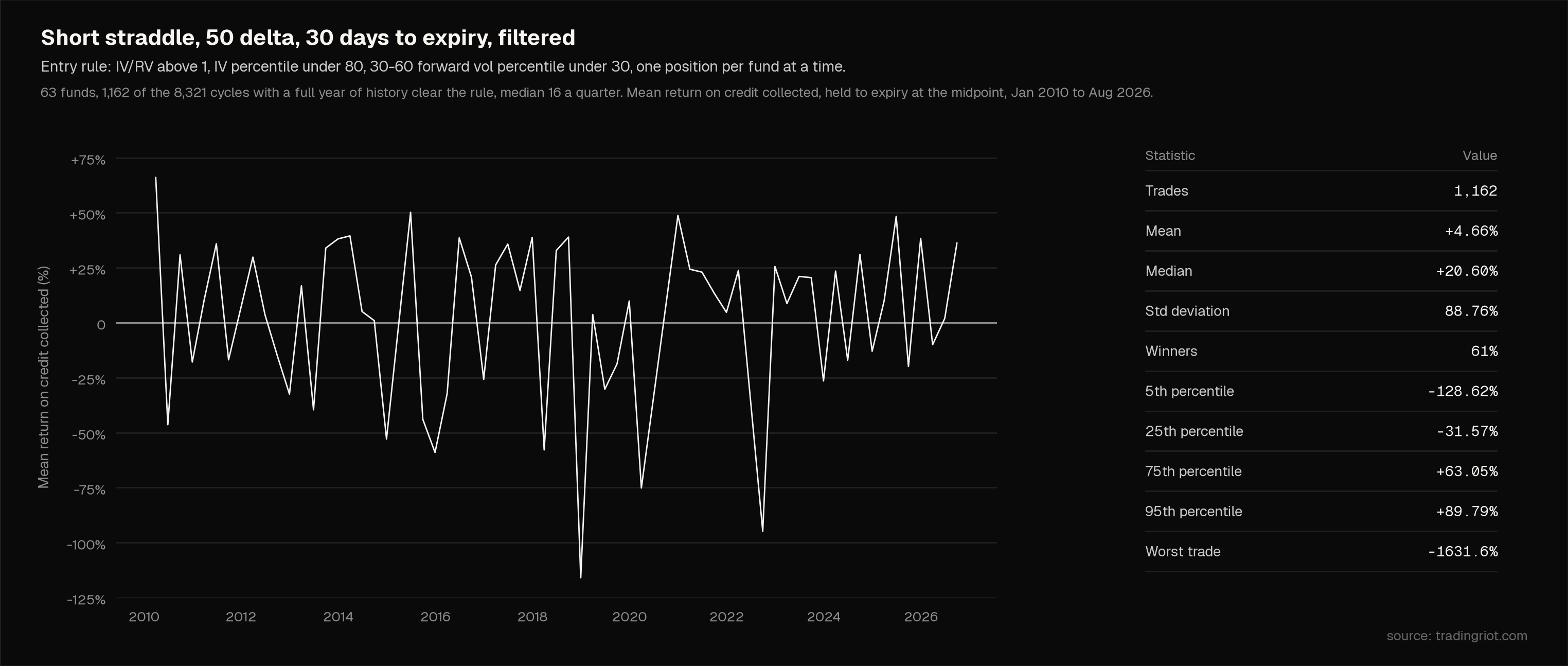
Looking at the chart above, the number of trades on straddles dropped from about 8,400 to 1,150, and the mean per trade improved, but the worst trade is still there.

This is still good. The original blind straddle was trading far too much, around 500 trades a year. Now it is closer to 70.

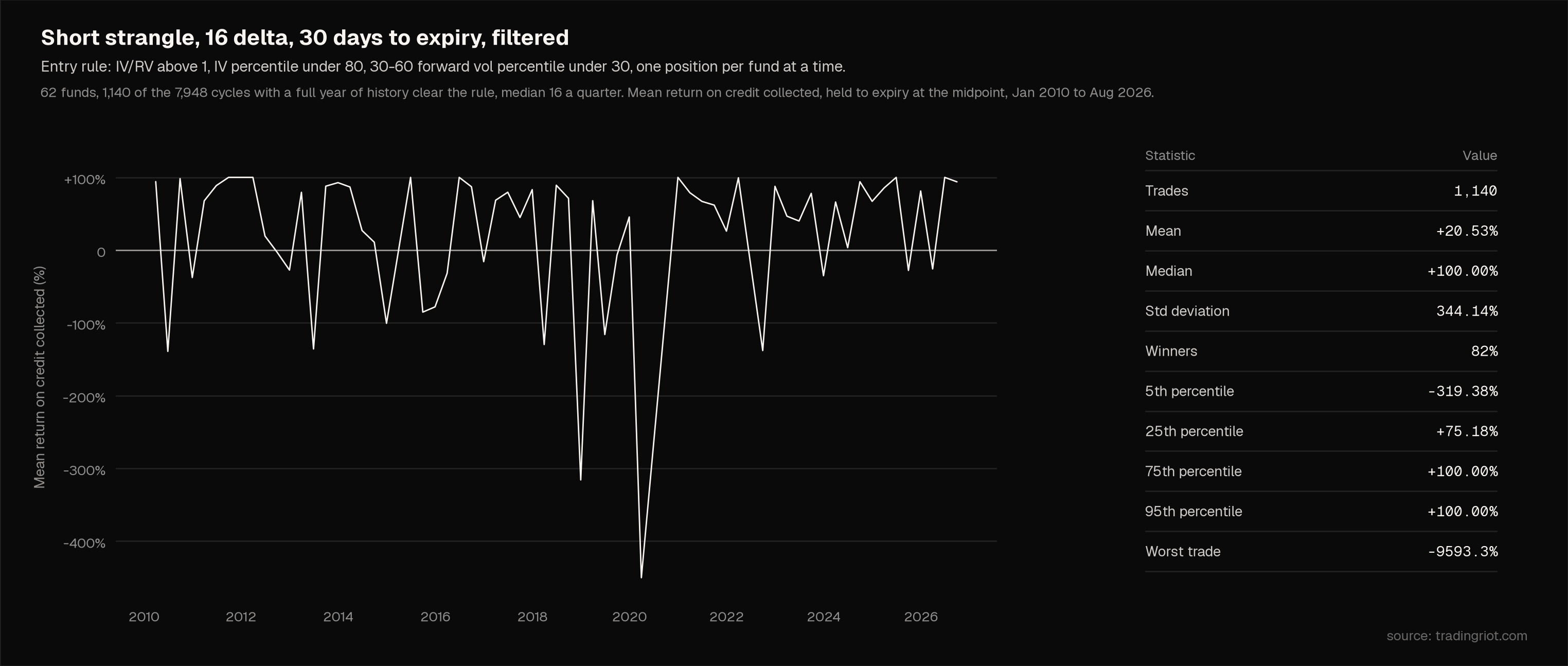
Returns on strangles also improved quite well on way fewer trades, but the worst trade is still there.

While the returns are great, I am not sure about you, but I do not personally feel like taking a trade with negative 9000% return potential. This is where we need to be careful, though; there’s a huge difference between calculated protection and being a pussy looking for favorable risk to reward.

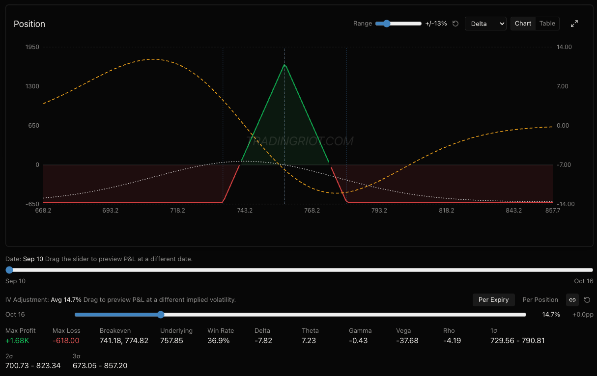
Here is a clear example of what trade with “favorable” risk/reward looks like: the 50/25 butterfly on SPY showing a max profit of $1.6k against a $600 loss.

I see structures like these often when I look online at volatility selling content on YouTube, but here is how this actually performs through time.

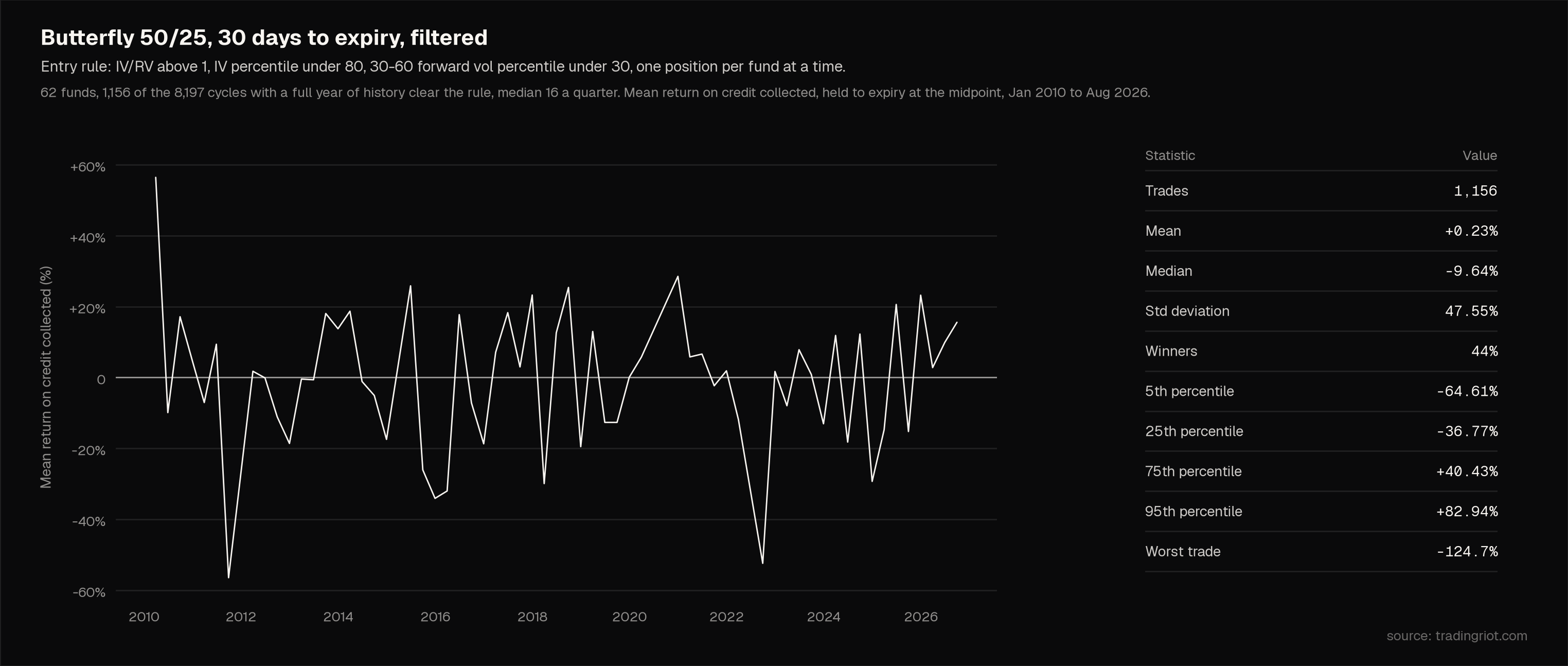
While the worst trade is not capped at -125% (which is slightly better than -9000%), the mean also collapsed to about 0.23%. This clearly tells us that selling butterflies with 25-delta wings won’t make enough money to compensate for the risk protection.

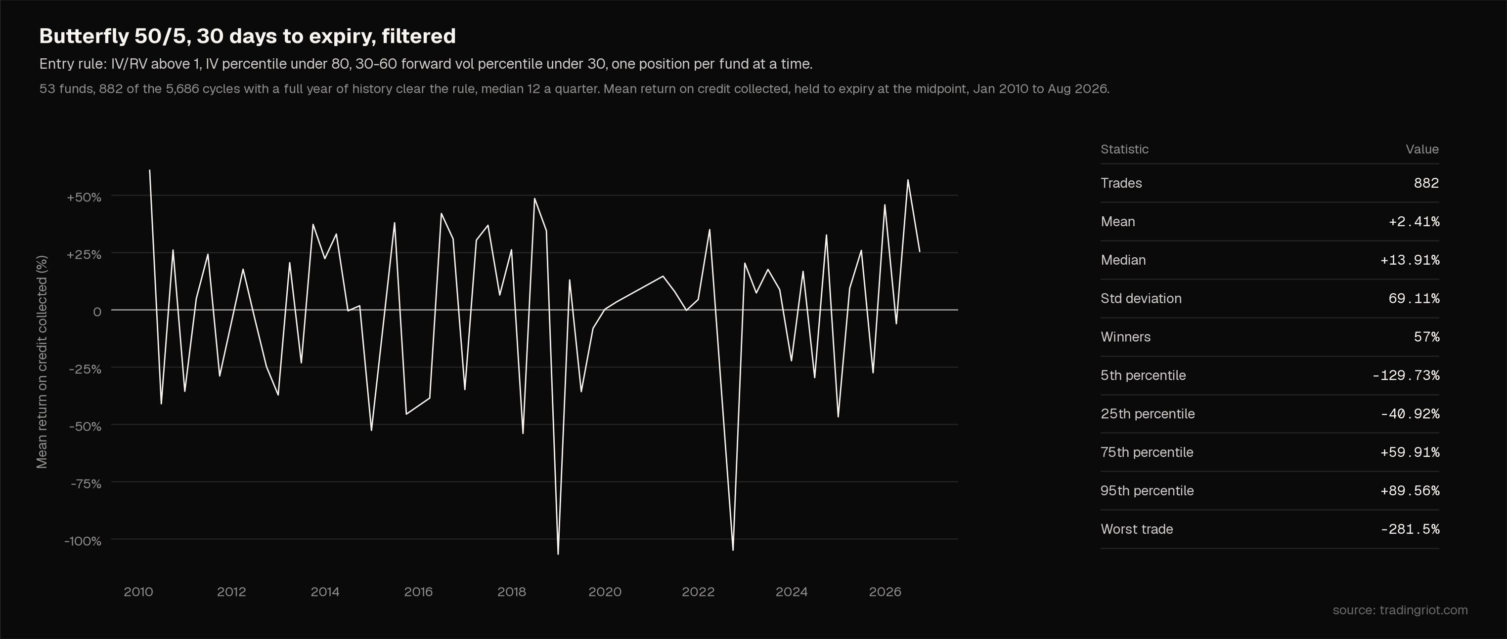
Here is the butterfly with 5 delta wings. I also added a rule that the credit cost can’t be more than 10% of ATM sales; this is why the number of trades dropped slightly.

Compared to straddle, the worst trade drops significantly, but at the same time, the mean drops as well. We will see in later on if this is enough to survive.

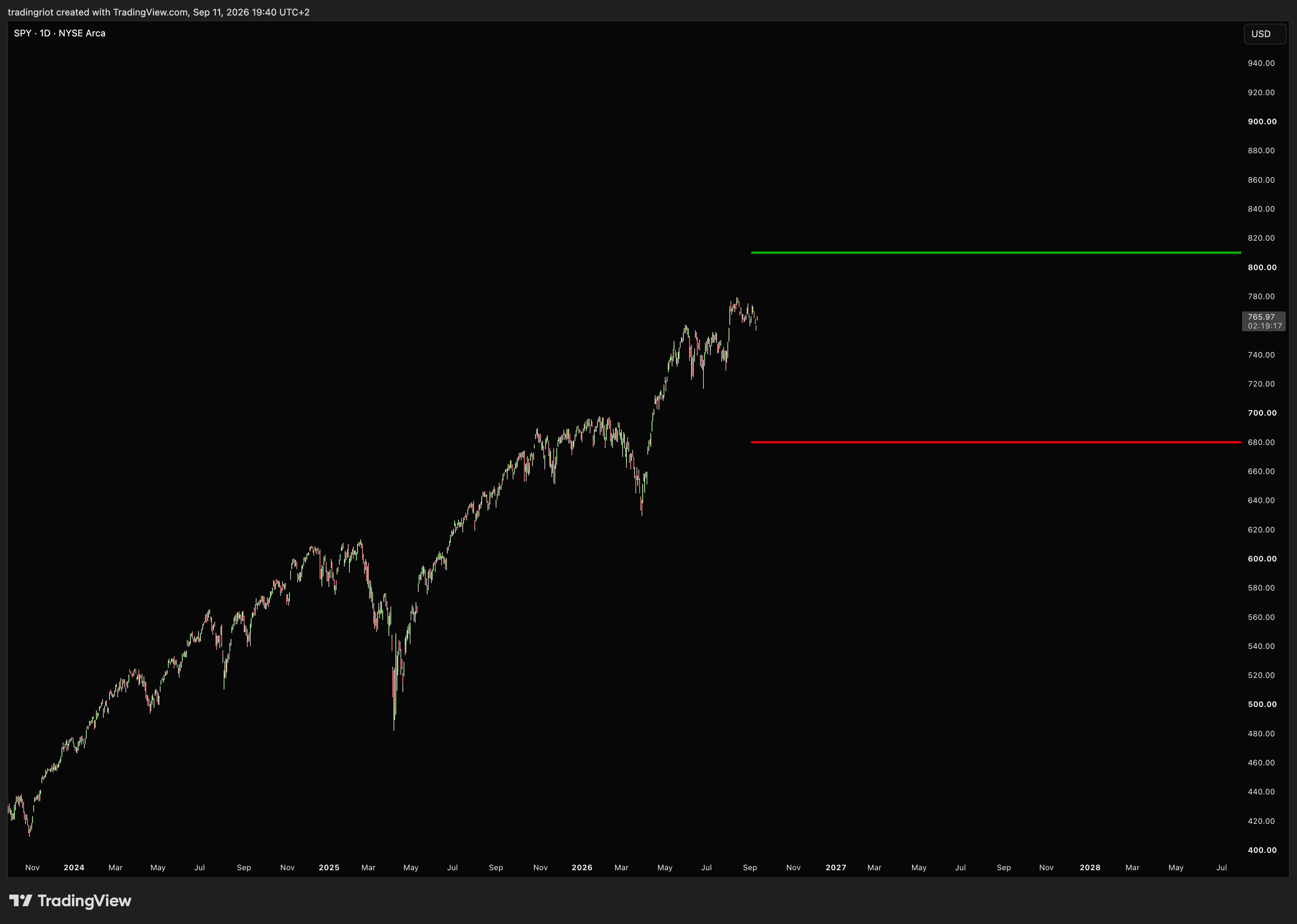
For reference, as of writing, the 5 delta wings on SPY expiring in 36 days sit at 680 and 810 with the spot at 765. The put is over 10% below the market, and the call wing is about 5% higher, because put skew means a 5 delta put is priced at a much higher implied volatility and therefore sits much further out for the same delta. The downside wing is in large crash territory, and the upside would need an aggressive drift to be breached at all, either of those is not something that happens every month.

So wings are really protecting you from something like two standard deviation moves, and if you try to buy wings closer to the price, you are buying options with inflated implied volatility because of the skew, so you are paying a variance risk premium to someone else.

How to survive

We went through a lot at this point; we set up our filters, tested different structures, and tested buying protection, so now it’s worthwhile to actually see how actual trading would look.

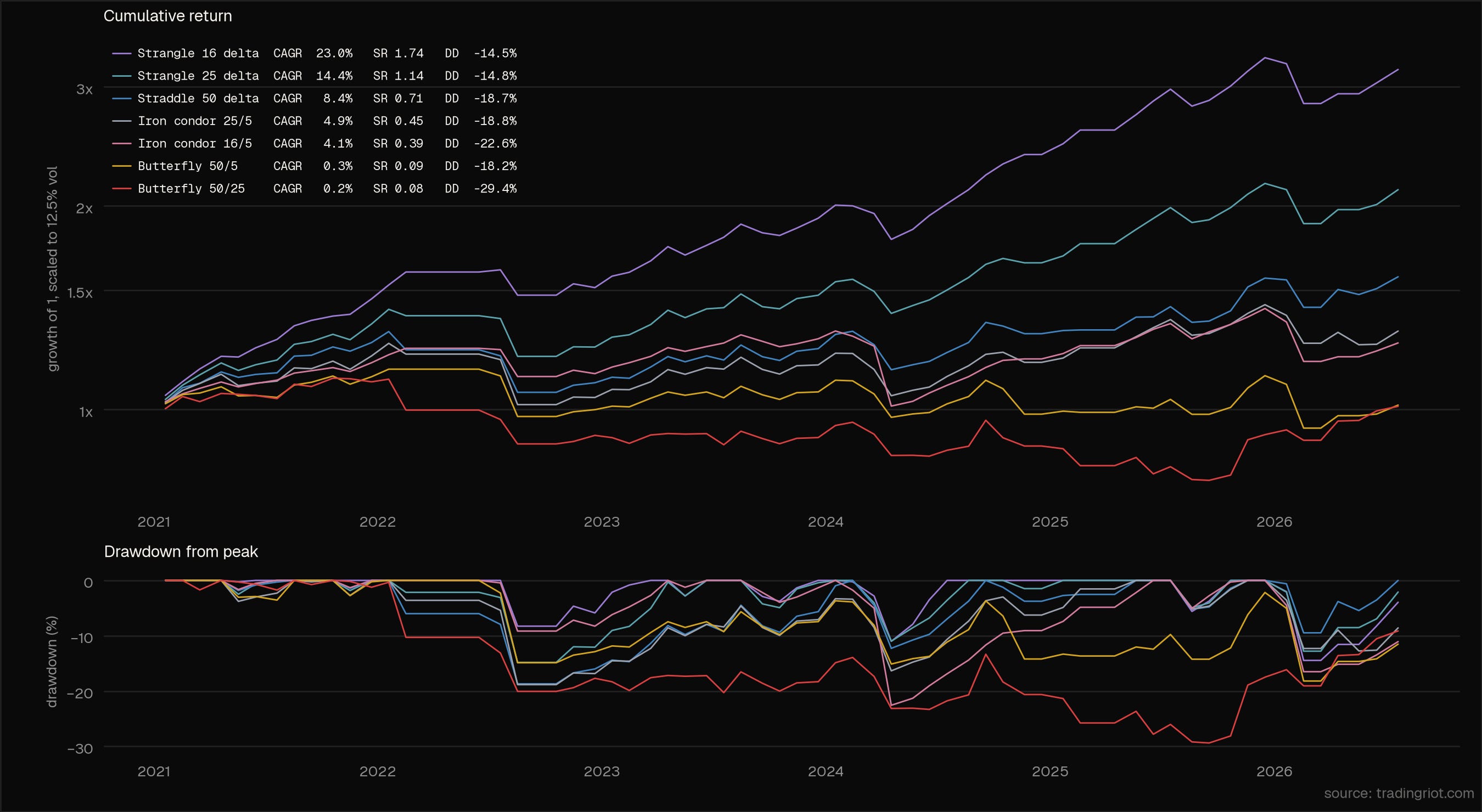
Pretty sweet, you can see I was right. Strangles are best; buying wings sucks. It did pretty well during the 2022 bear market; you should just run it and call it a day, right?

Well, unfortunately, thanks to Wuhan, five years of data are not really enough to be confident.

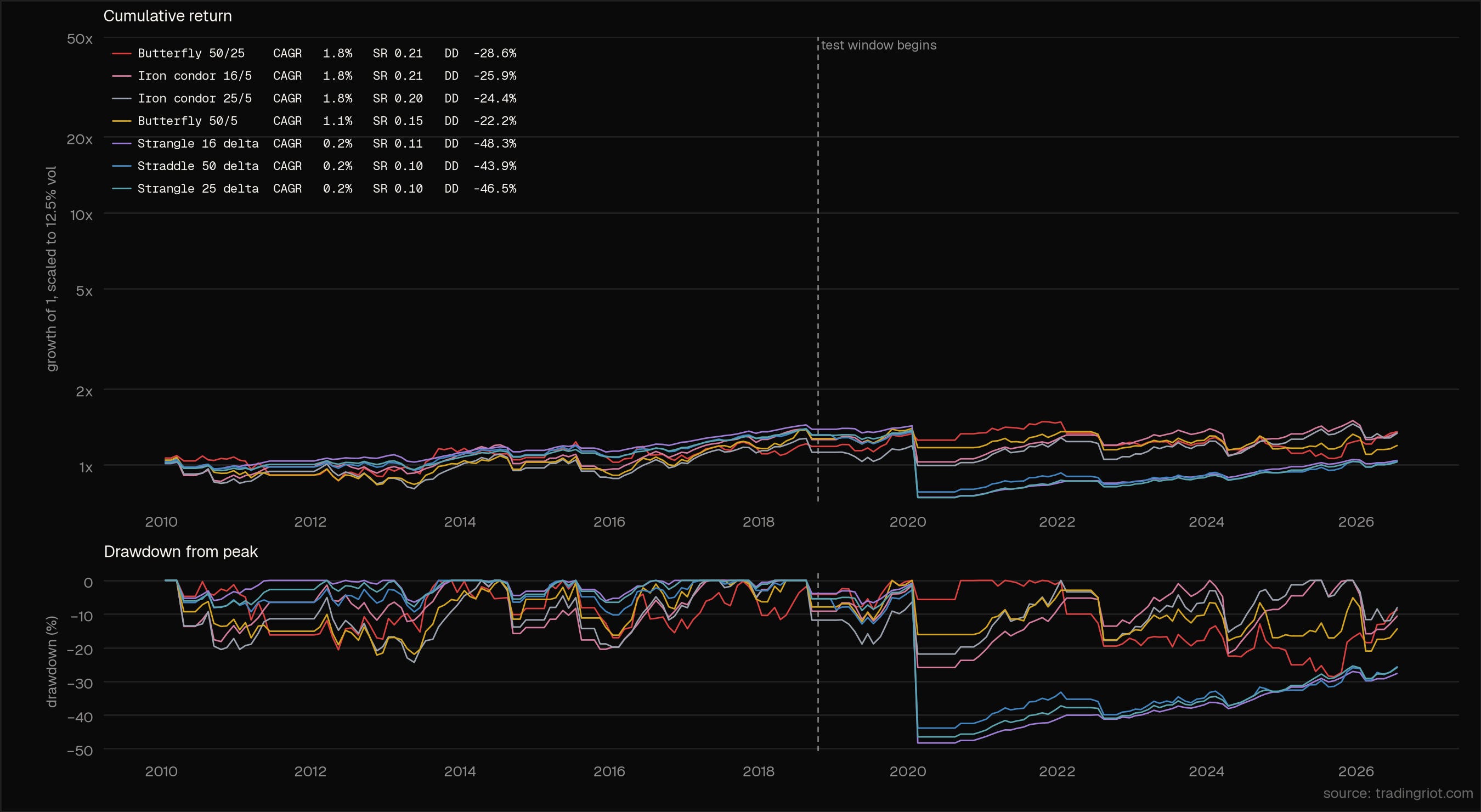
Before I talk more about this abomination, I’d like you to know that this backtest covers just over 16 years, January 2010 to August 2026, selling volatility on 114 plain ETFs whenever the three conditions are met alongside a volume filter of 10,000 contracts traded on a 20-day average (dropped to 5,000 contracts during the early years).

Tested on actual bid-ask data with entry is priced a quarter of the way in from the ask price, which is better than the midpoint, so the fill assumption is on the generous but doable on liquid ETFs, with trading commissions also included.

Trades target 30 days to expiry on standard monthlies and are accepted between 21 and 45 days. Each one is held to expiration and settles at intrinsic, so no spread is crossed on the way out.

While a position is open, no new trade is taken in the same instrument. Every series is scaled to a 12.5% annualized volatility target, which is a sensible level for a negatively skewed strategy.

While this does not include some edge cases of assignment, I would say it doesn’t matter anyway because you would still probably be licking your wounds from 2020 anyway.

I have mocked James Cordier through out this article only to ended in same position like him, this is the whole problem with selling volatility in markets that are often correlated and when shit hits the fan it often hits acrross the board.

But we are not giving up here, as I mentioned at the beginning of the article. I have a consistently profitable strategy, which I still intend to share, but before you are ready for that, you need to be able to see some pains and understand why certain things don’t work.

Delta hedging

We only looked at two scenarios, buying protection for catastrophic events or not buying it at all, but most trades will end up somewhere in the middle with prices just wiggling around through out the time of the option.

When you buy an at-the-money call, you are buying an option with a 50 delta; in other words, the option behaves like being long 50 shares of the underlying. For buying an ATM put, it’s about being short 50 shares.

Since we are selling options, this flips with ATM calls having a -50 and puts a +50 delta. If the underlying is trading at 500 and you sell both ATM call and put, you have a straddle, and at the open these two deltas cancel each other out and your position starts with a delta of zero.

This is precisely what we want since we are not speculating on price movements but on volatility, but unfortunately for us, markets are moving, and the next day the underlying is trading at 515.

The call you sold yesterday is worth more and has, let’s say, a -65 delta, while the put you sold is worth less, a 35 delta. You are now short 30 delta, which is something you don’t want; you want to avoid exposure to the underlying; you only care about the fact volatility is rich.

So you buy 30 shares to flatten out your delta. The day after, the underlying drops back to 500 again; your delta is zero, but you now have 30 shares; therefore, you have to sell them for a small loss.

Delta hedging must be pretty familiar to most of you since it is evolving to often buy high and sell low for a loss, but this is a necessary process to have no directional exposure.

Hedging is not always loss-making if the underlying rallies to 535 and expires there. Assume you sold a straddle for $20, but the call expired at 35, so you lost 15 ($1,500) on one straddle, but the 30 shares you had bought on 515 are now worth 20 points per share, so $600 is reduced from the straddle loss, and had you kept hedging as the delta grew past 30, you would have recovered more than that.

delta on a short straddle

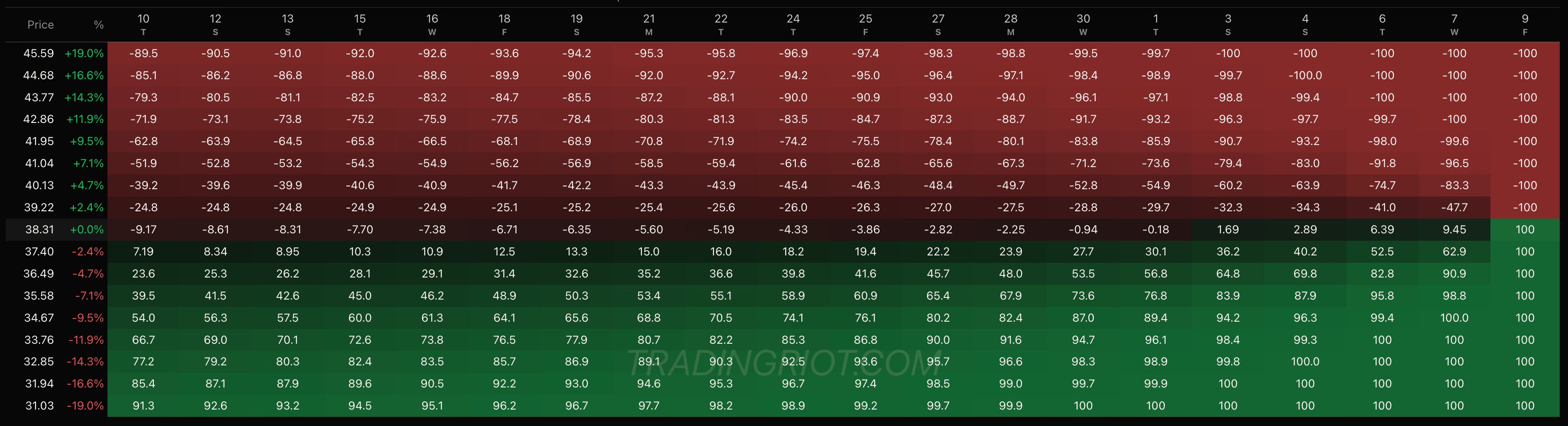
So we can just hedge nonstop right to fully remove the directional risk and live happily ever after? No, not really; trading costs money.

If you over-hedge, you can easily spend a large part of your premium on trading costs, making the whole strategy unprofitable, but hedging too little is also not the best since you are exposing yourself to large moves.

Some traders hedge once per day or per week on longer positions, or what I think is more reasonable is to set fixed delta bands and re-hedge to zero once these are breached.

From the example above, let’s say your delta bands would be at 30 delta; therefore, you would hedge only if the underlying moved to 515 and do nothing if it wiggled between 486 and 514.

The issue is that this number is arbitrary. Is the 30 delta band better than the 20 delta band, or maybe the 40 delta band is the best one?

Luckily for us, someone much smarter looked at this problem before; in 2006 Valeri Zakamouline published a paper called Optimal Hedging of Options with Transaction Costs, which I read about in Euan Sinclair’s book.

Using some simple elementary school math, we can calculate the band:

band = H0 + H1

H0 = λ / (γ · S · σ² · T)

H1 = 1.12 · λ^0.31 · T^0.05 · (e^(−rT) / σ)^0.25 · √(|Γ| / γ)

S is the spot, σ the implied vol of the position, T the time to expiry in years, r the risk-free rate, Γ the position gamma. The two you choose are λ, the cost of trading the underlying as a fraction of notional, and γ, how averse you are to risk.

H0 is the pure cost term. Cheap execution or a big, fast-moving, long-dated position makes it small, so it hardly matters most of the time. It blows up in the last few days before expiry, when T in the denominator goes to nearly nothing.

H1 is the term that does the work, and the only input that really moves it is gamma. Bigger gamma, wider band.

That might sound weird, as you would probably expect hedging more with large gamma, but the delta is moving so fast that any level you hedge to is stale within hours, so tightening the band just buys you more trades at worse prices for the same exposure.

Zakamouline’s answer is to stop being a pussy chasing and carry the drift instead.

If we use it in an actual example of a 30-day ATM straddle on our 500 underlying with 20% vol:

Γ (position): 0.0278 per share, 2.78 per contract

H0: 0.0061

H1: 0.1043

band: 0.110 = 11 shares per contract

So you do nothing while the position’s delta sits inside plus or minus 11 shares a contract, and when it breaks out, you flatten.

That is roughly a third as wide as the 0.30 fixed band most people use in this position, at this vol.

30DTE, Γ 0.028, band 0.11, 11 shares per contract.

14DTE, Γ 0.041, band 0.135, 14 shares per contract.

5DTE, Γ 0.068, band 0.186, 19 shares per contract.

1DTE, Γ 0.108, band 0.389, 39 shares per contract.

Vol pulls the other way, because a higher implied vol on the same strike means less gamma. At 12% the band is 17 shares, at 20% it is 11, at 40% it is 6. A high-vol name gets hedged tighter than a quiet one, which is the opposite of the instinct.

No need for a panic attack now; I have built this as a calculator on my website inside the Position Builder and calculator section so all the math is done for you.

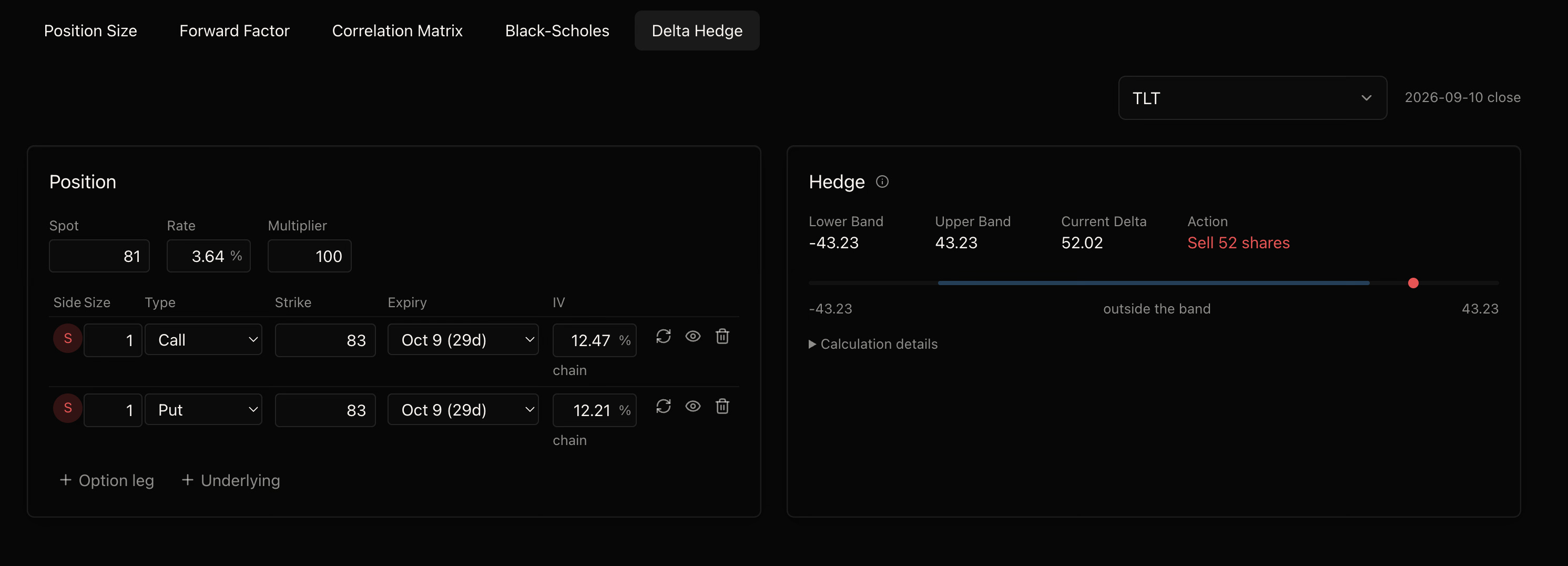
There is one nuance worth knowing: Zakamouline’s original paper is hedging back to the band edge as it is for intraday trading. Since I trade long-term positions at EOD rebalancing, I am hedging back to zero delta instead.

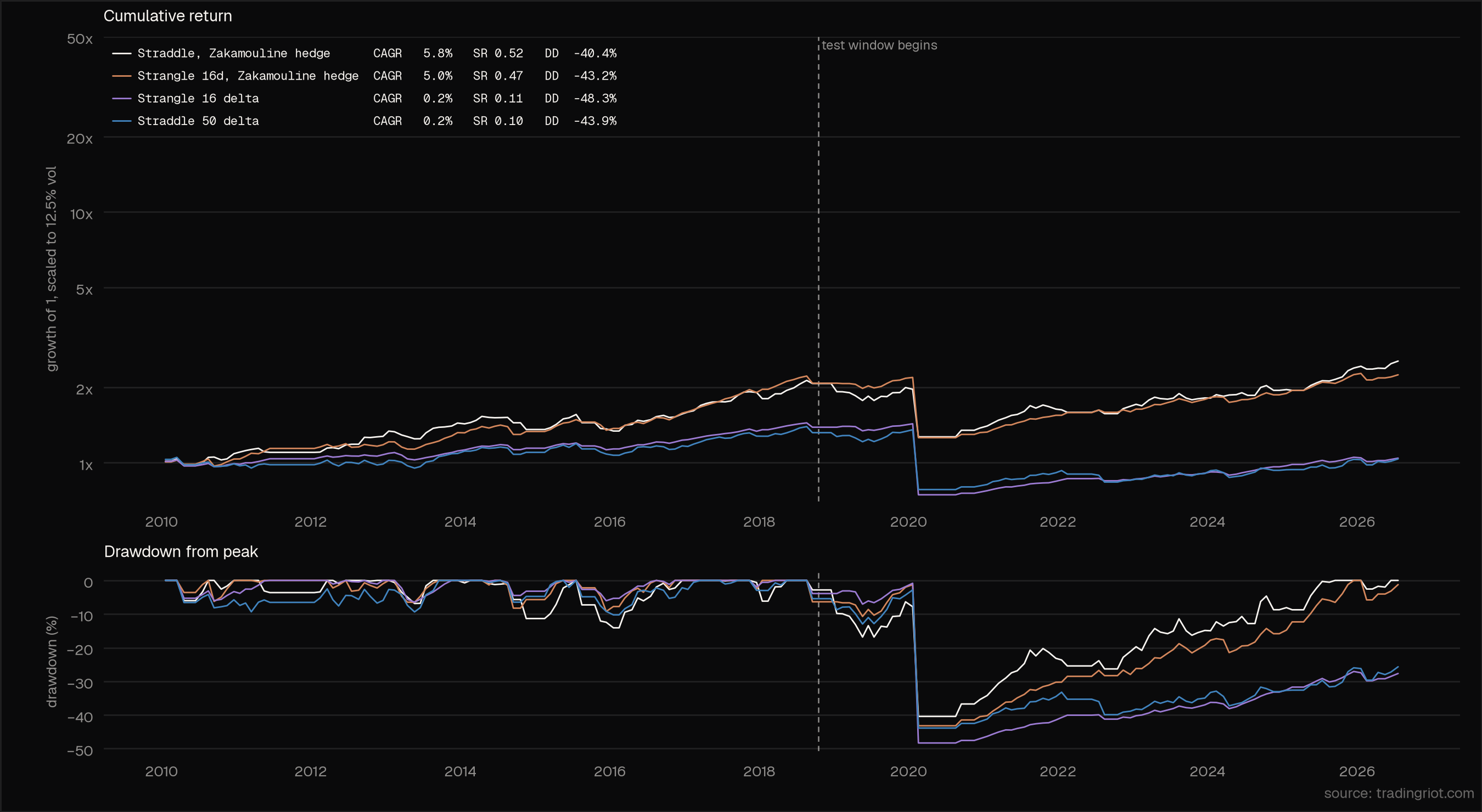
It’s better, alright?!

Unfortunately though, delta hedging would not save you from COVID either; hedging is going to save you from the drift, but when the market is crashing 10% overnight and going limit-down, no amount of EOD delta hedging wont help.

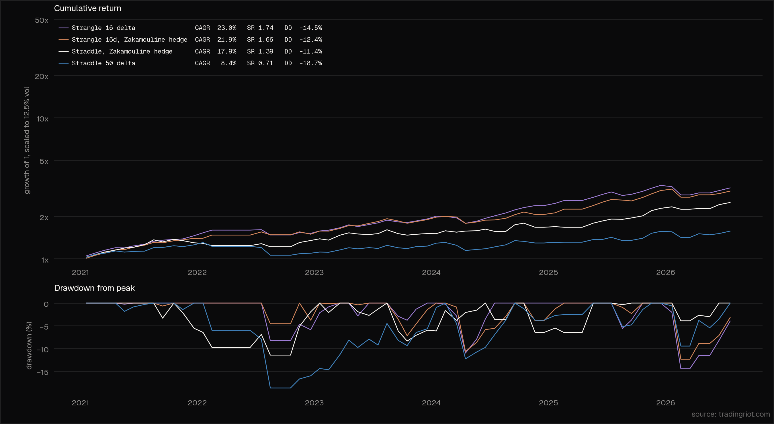
Using a more convenient data set from 2021, you can see that delta hedging beats the naked straddle, and while it doesn’t beat the naked strangle on raw returns, it provides slightly lower drawdown and a smoother ride.

Understanding how delta hedging works and being able to utilize it is generally a useful tool; also, if you for whatever reason want to sell a straddle or walk your entry from 16 delta closer to ATM, your returns will improve if you delta hedge your positions (and there won’t be an end-of-world scenario in the following thirty days).

When music stops

I think it is pretty clear at this point that the only way to save ourselves is to exit trades early.

One of the first things that we have done is finding rules to predict the when subsequent realized volatility will be muted, we have also noticed that when those filters were at opposite extremes the volatility heavily incresed.

The forward volatility rules look at what the market pricing is for the month after the expiration and take trades only when calm conditions are expected. If, during the trade, the thirty-day rises above the sixty-day, the curve has inverted.

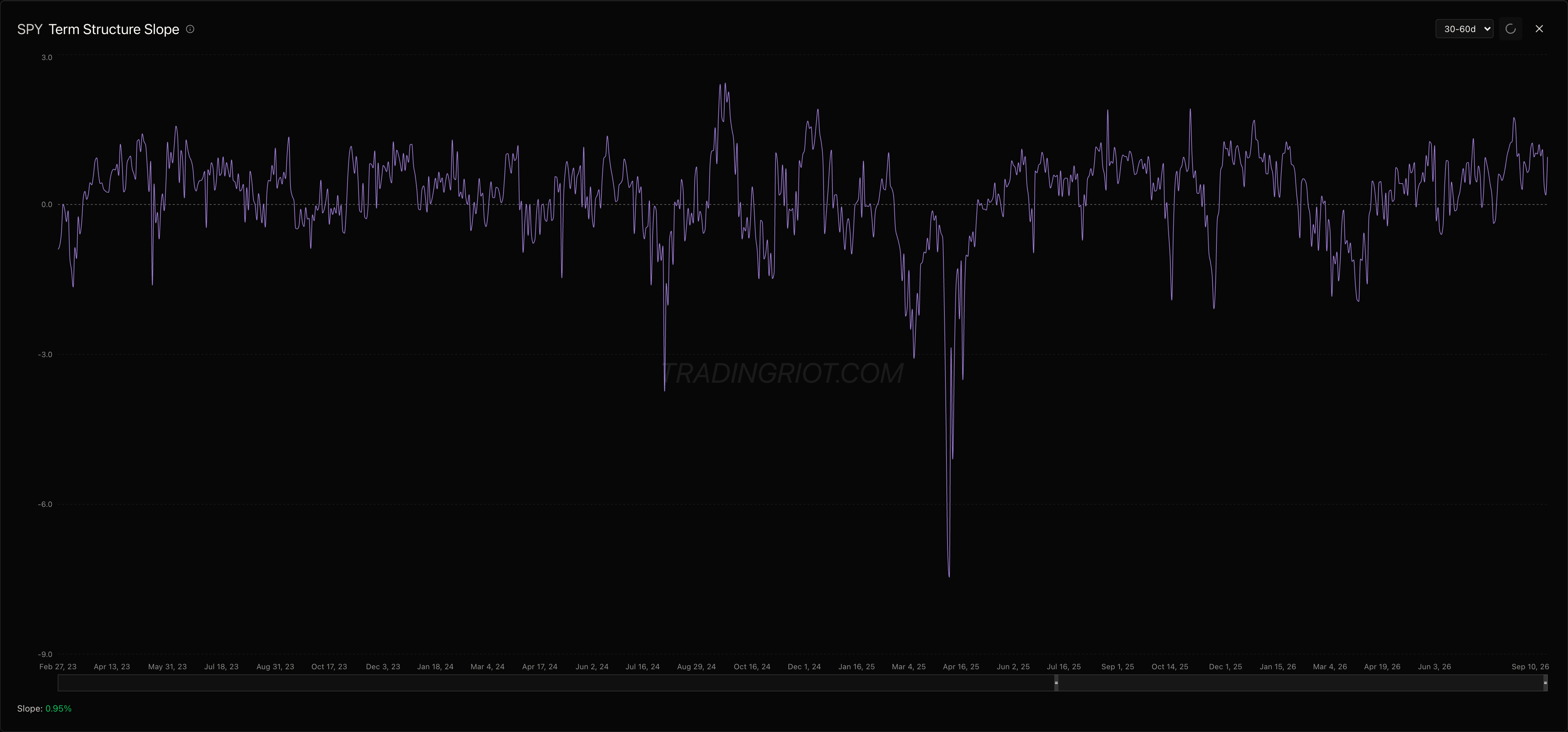
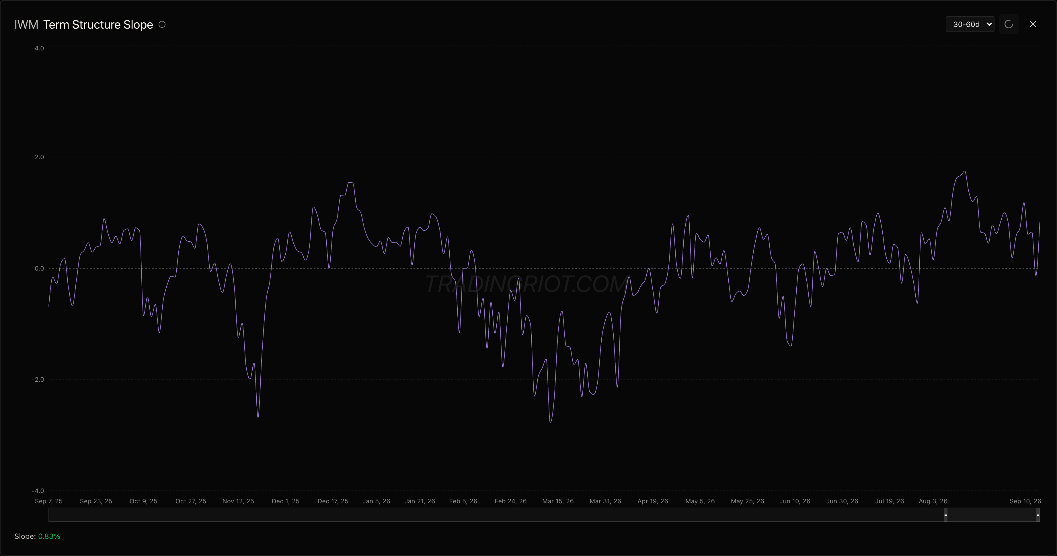
This is what the term structure slope measures: you take the 60-day IV minus the 30-day IV. If the number is positive, the curve is in contango; if negative, it is in backwardation.

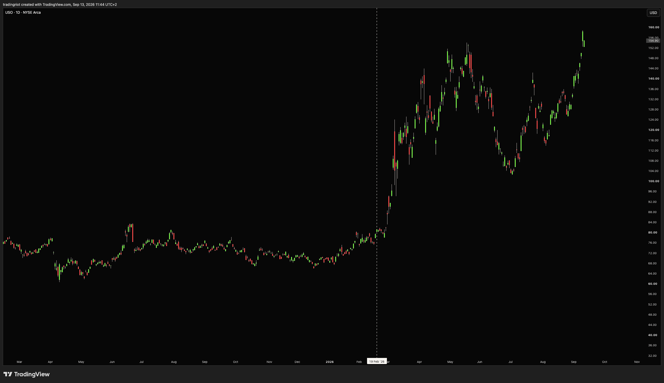
On SPY, the curve went to backwardation on February 19th, right before the selloff happened.

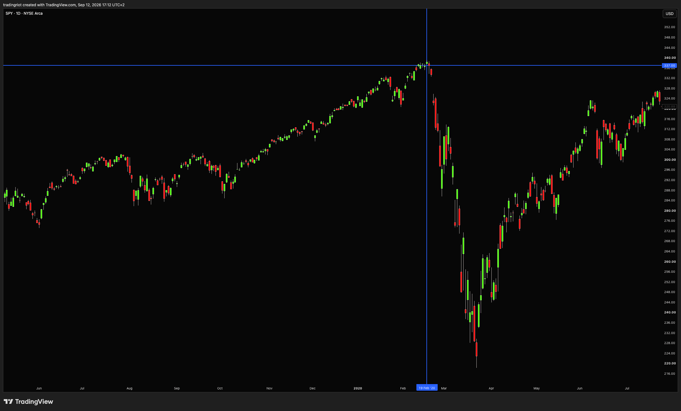
Therefore, our new rule is simple: enter trade only when the ETFs’ 30-60 day term structure slope is in contango (above 0) and exit the trade if it gets backwardated (below 0).

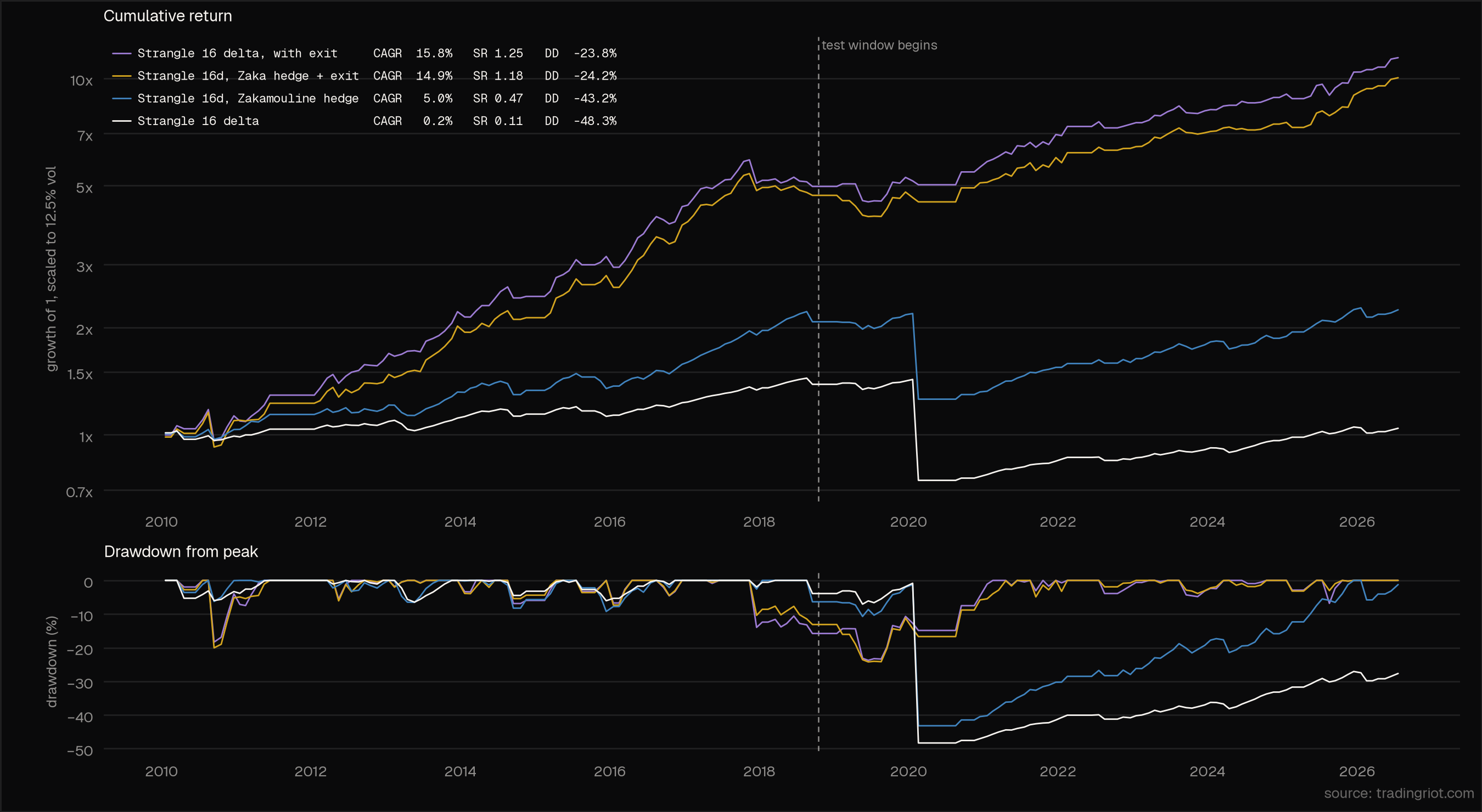
The early exit is what saves us; it is worth more than buying wings and more than hedging. You can see their downside by looking at 2021 onwards.

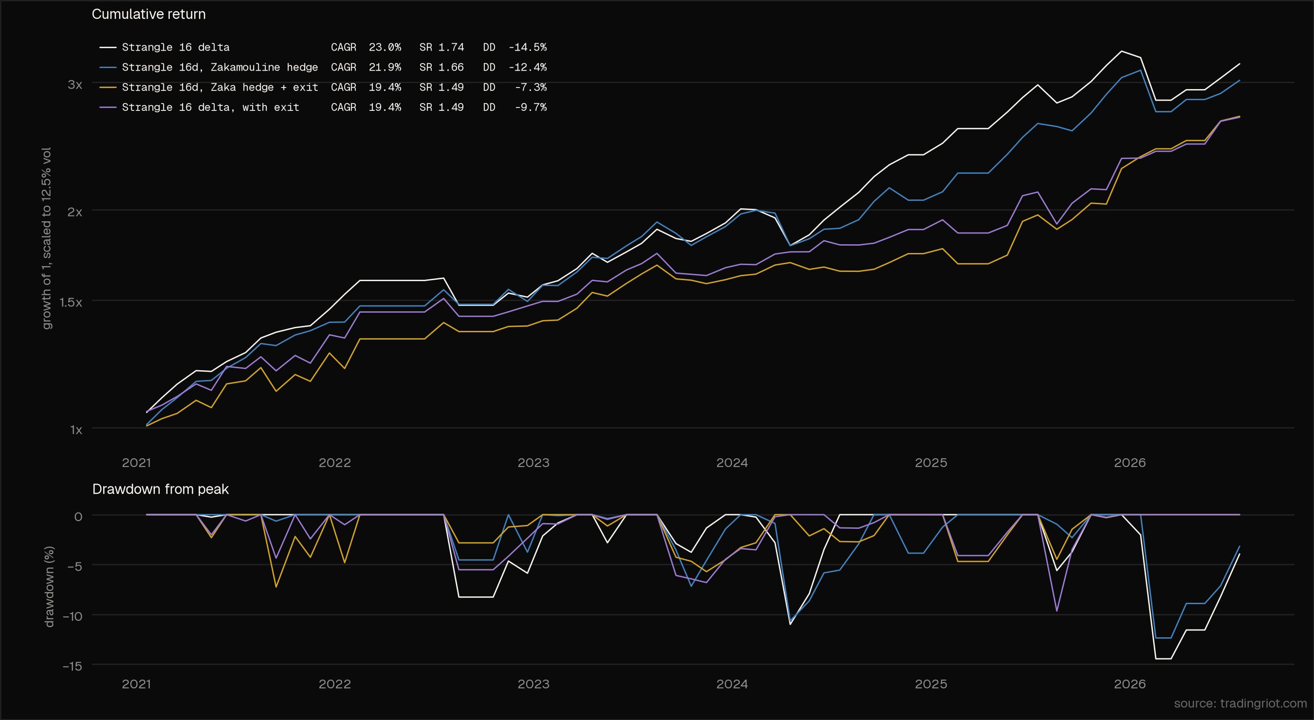
They are not free; from the whole backtest, they only ever saved you during COVID. In other market conditions, hedging or just holding a naked strangle was better.

The whole strategy changes a lot; about 75% of trades are exited before the expiration as markets often go backwardated during small signs of stress. If you hold to expiration, you are not crossing the spread on the way out since settlement is not a trade; now every early exit costs money.

This was modeled into a backtest, but the same as the entry at 25% from the ask, exits should be started at the bid and walked to the mid. Since most of the signals are not leading to the end of the world, I believe this is doable with liquid ETFs, but you should be extremely mindful of trading costs when dealing with options.

The real world

While I kept the backtest as true to the real world as possible, there is always more variance when it comes to actual trading.

There might not be an actual 16 delta strike available, you won’t be able to afford the position due to high margin, and so on.

This is the type of strategy that I prefer to trade manually after it has been verified in a backtest rather than trying to fully automate it. This allows me to use some discretion when it comes to execution and the number of markets concurrently opened and so on.

One of the other reasons why we prefer to sell strangles is because of skew. As I mentioned previously in the article, not only do different expirations have different IVs, but different strikes also have different IVs; this is called skew.

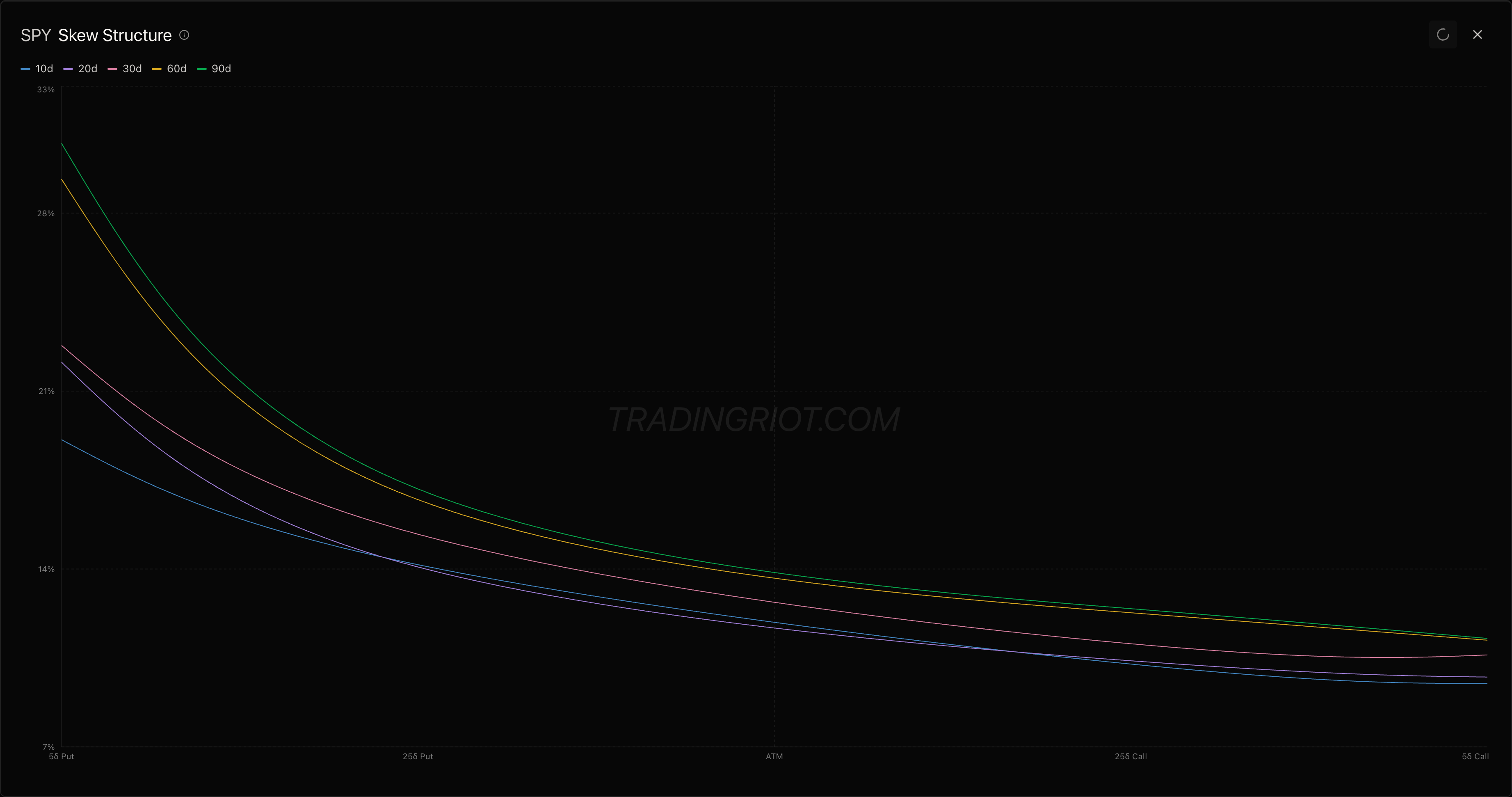
Equities have persistent put skew driven by demand for hedging; commodities, on the other hand, might have positive call skew due to supply shocks.

While you are never going to get the same credit as for straddle, elevated skew richens the wings, so your credit gives you a decent premium considering wider breakevens.

We also need to understand the spot-vol correlation. Plenty of markets we are going to trade have high spot-vol correlation, mostly negative.

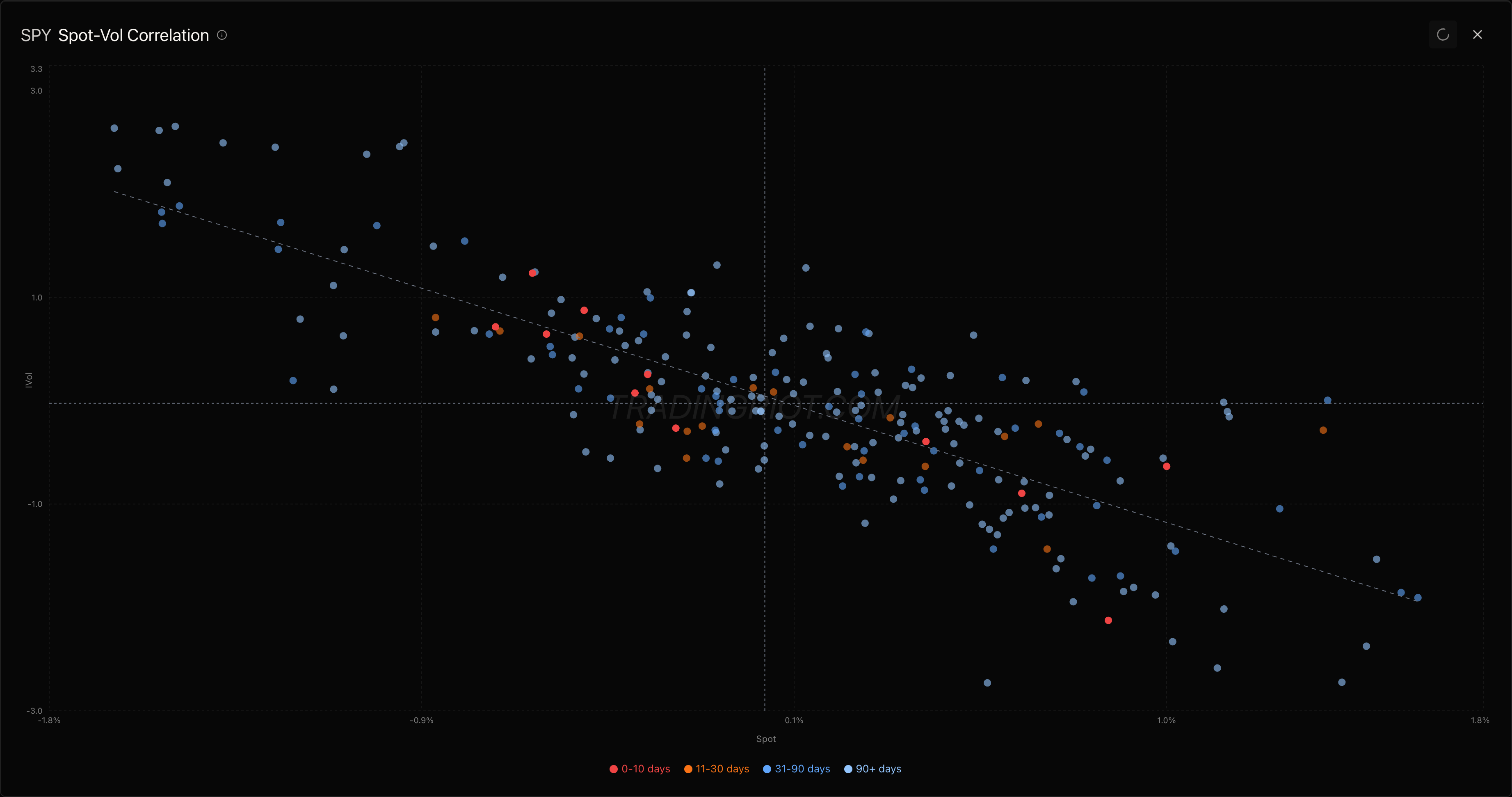
This is what is called “shadow delta” when price drops, IV tends to rise and vice versa. When this happens, options delta is not only changing because of price change but also because of IV change.

Equity markets especially have positive drift; if you are going to sell straddles, you can place short strikes not ATM but slightly above; therefore, you are not going to have to delta hedge when the price drifts upwards, and you will also benefit from a drop in IV if the market rises.

If you are trading strangles, you can also shift your strike based on skew to position slightly better for a positive drift.

For example, instead of selling 16 delta strangles on QQQ, you can shift your strikes slightly higher so the structure is more 20/15 delta, and you are entering a trade with slightly positive delta so you lean to the tendency for IV to fall on rallies.

20/15 strangle on left. 16/16 on right

Looking for trades

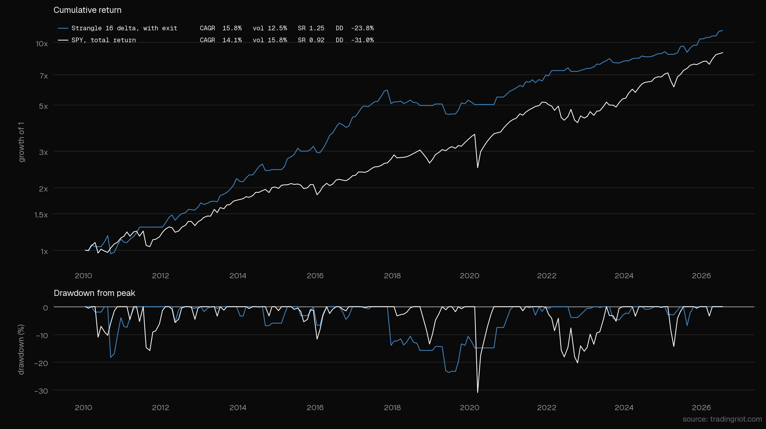
We are coming to the end. We established all rules and turned something that has a massive tail risk into a decent strategy, which beats the benchmark and deserves the place in a broader portfolio.

If you want to start the strategy yourself, you can use the Tradingriot analytics website to look for trades.

The short volatility screener is already pre-populated with filters we have established.

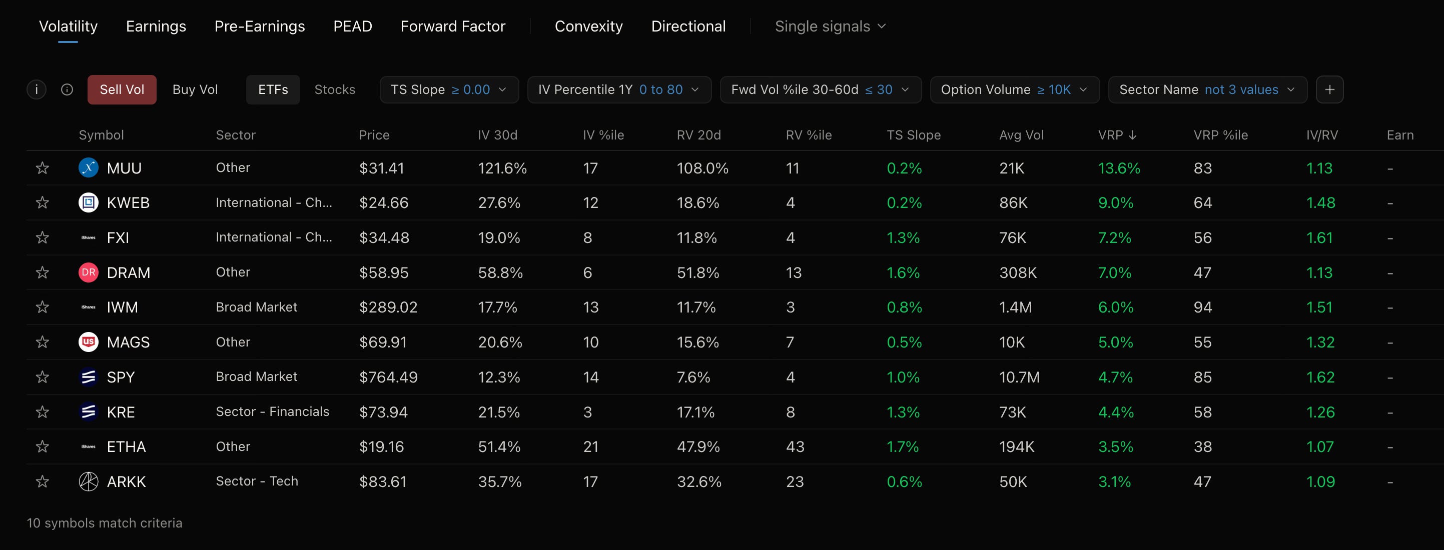
We can look at IWM as an example (while we ignore MUU, which is leveraged and slipped into the screener).

Volume conditions are not a concern here since IWM is trading 1.4m contracts on a 20-day average compared to a 10,000 limit; IV percentile is on the 13th percentile, well under the 80th limit.

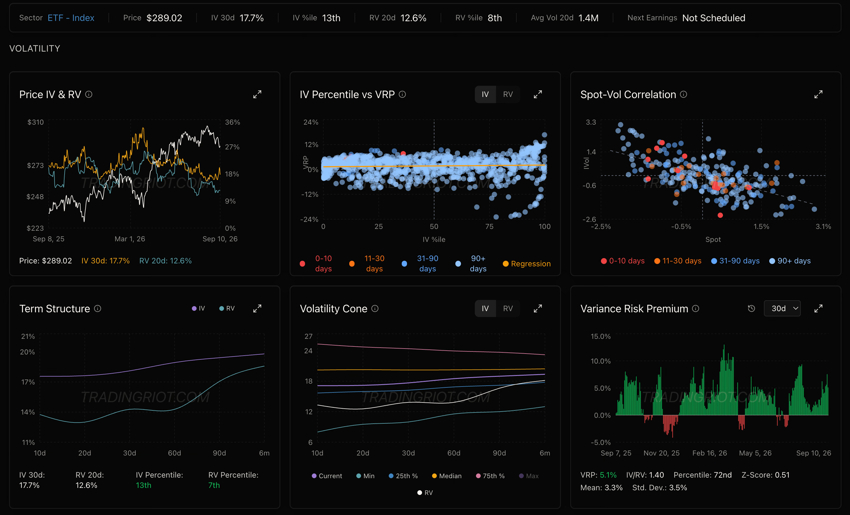
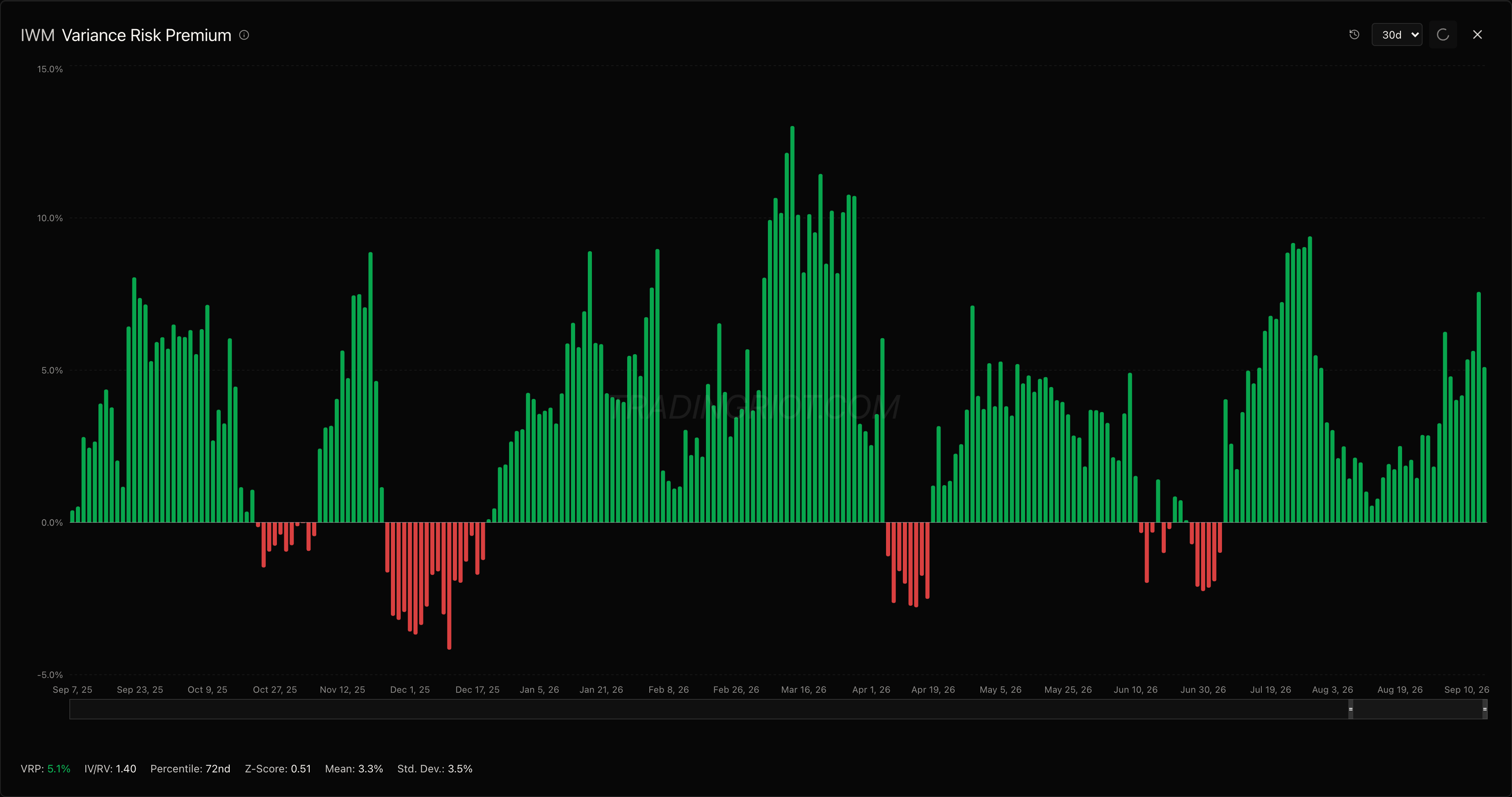
Variance risk premium is present, with the premium being 5.1% and the IV/RV ratio at 1.4.

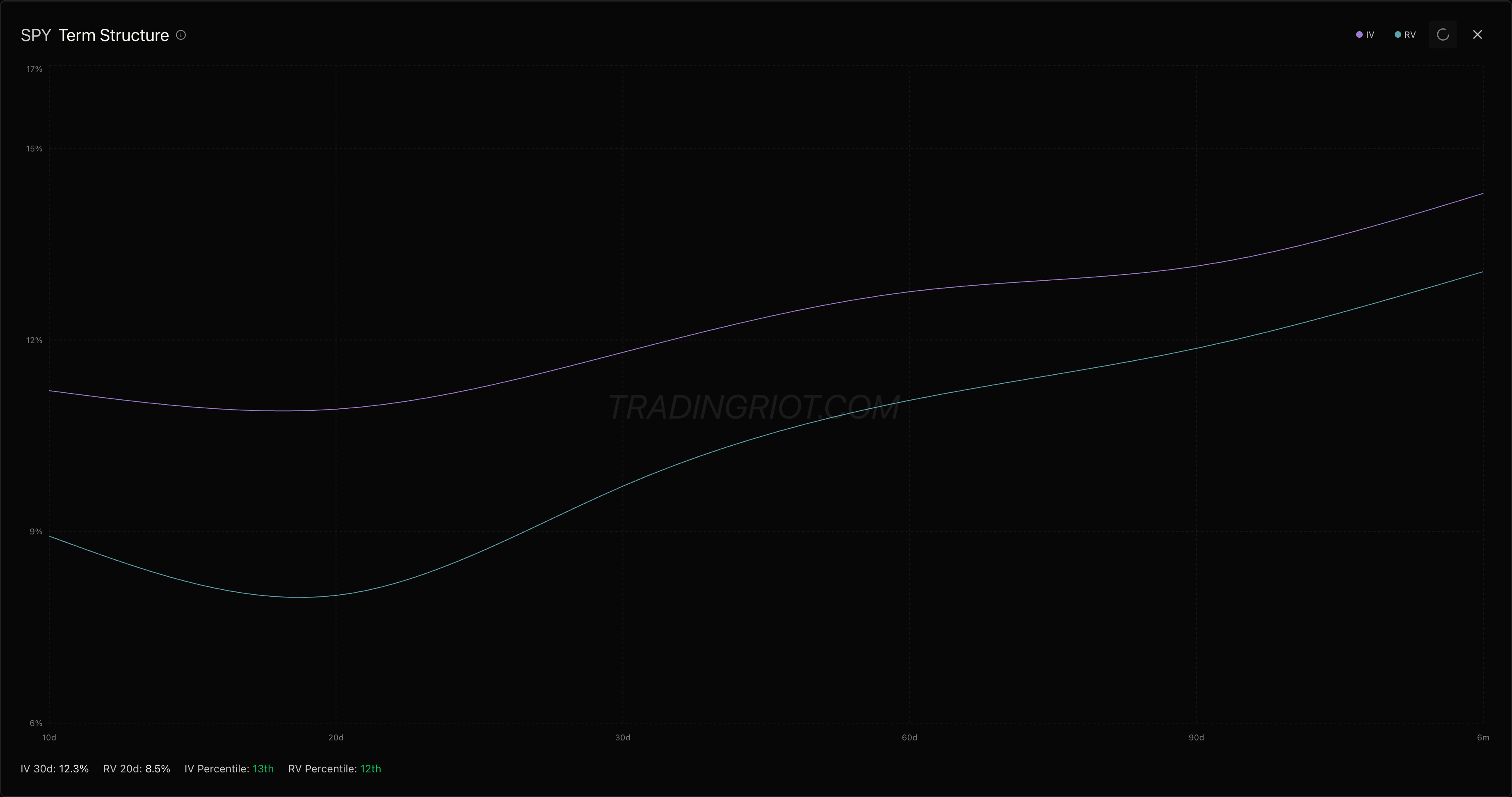
While short-term 10-day IV is elevated, the term structure slope condition is also met when looking at the difference between 30- and 60-day implied volatility.

The last condition is also met with forward volatility percentile at 16, so we can now look to structure the trade.

Now it comes to some discretion; you might have noticed that the screener showed SPY, IWM, KWEB, and FXI, among some other markets.

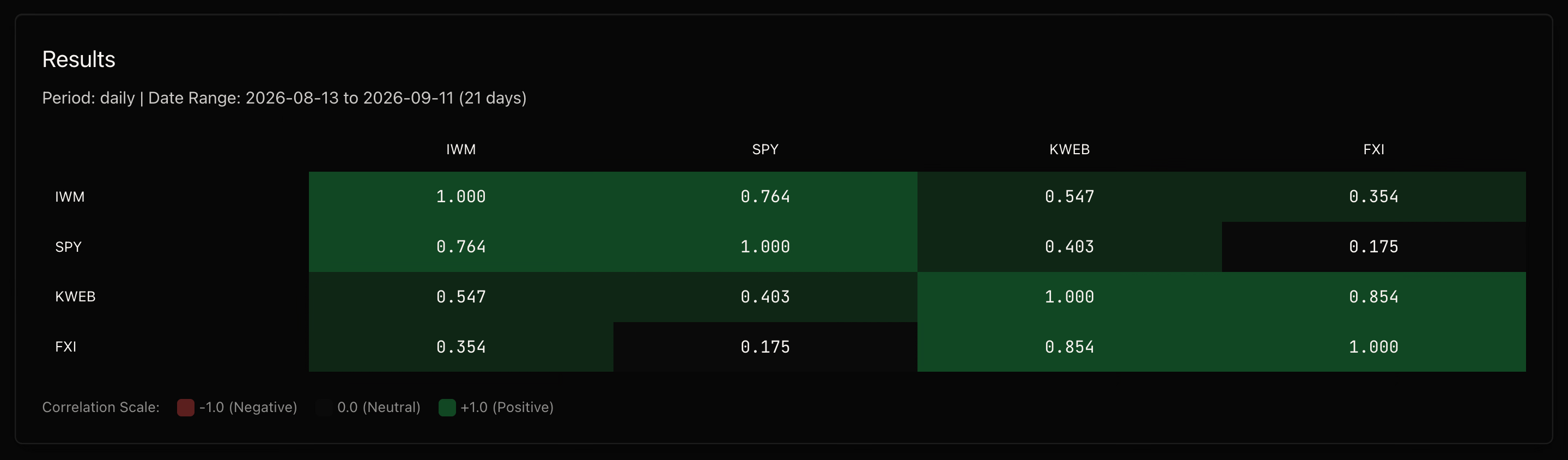
SPY and IWM are highly correlated, the same as KWEB and FXI. I tested correlation and how it affects performance, and having a book with lower correlation around 0.5 led to lower drawdowns. For that reason, I would not hold more than two highly correlated markets; for discretionary trading, I generally aim to have about 5 positions, ideally using uncorrelated assets.

Another thing you want is to give strangles some width; when IV is extremely low, usually under 10% in absolute terms is giving you very narrow strangles.

This is often an an issue on bonds where your breakevens are very narrow so any shock moves can lead to large losses

So if IV is under 10%, that translates to about 5-6% total width.

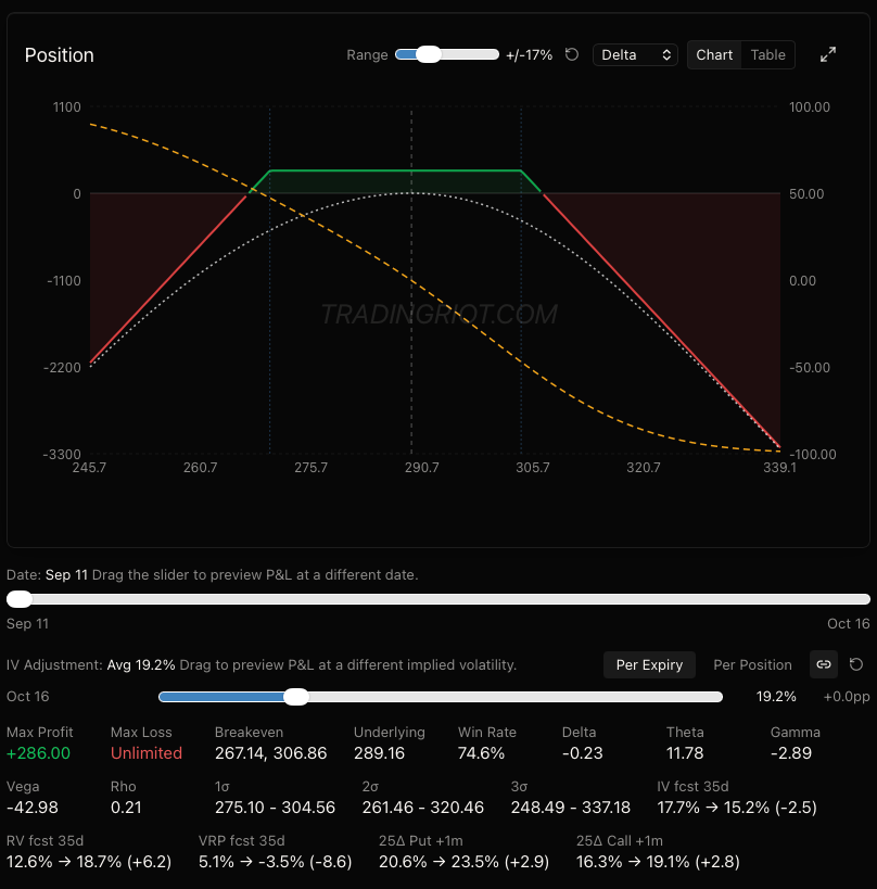
From this example, you can calculate width easily by (call strike - put strike) / spot, which in this case equals 11.8%, so comfortably above the 5%.

By the way, if you scroll through the position builder, you will see the exact percentage from the spot, so you can just eyeball the width by doing that.

When I trade these, instead of going for fixed 16 delta strangles, I am picking strikes by looking at the implied distribution.

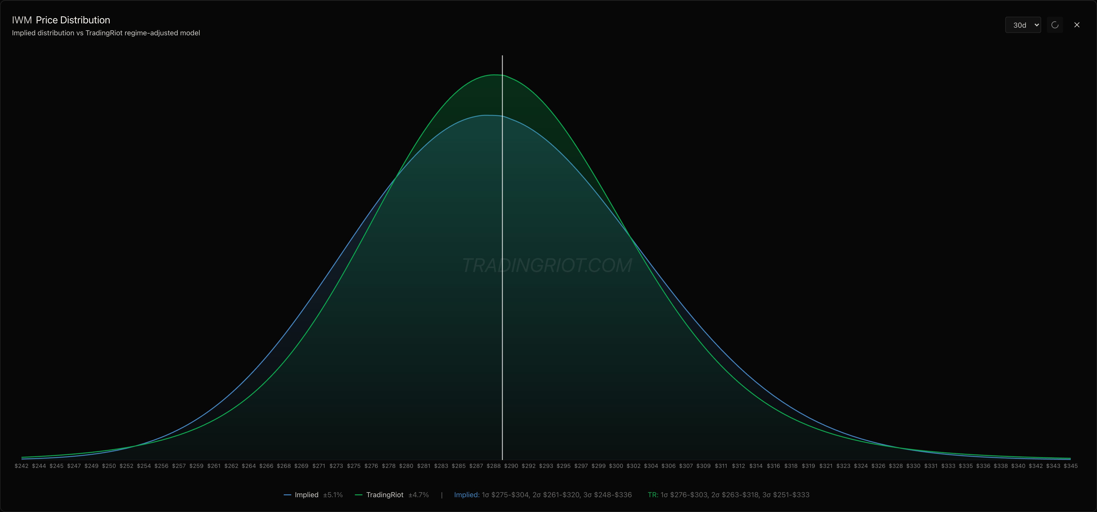
Above you can see two models, markets implied, which is simply based on implied volatility, and my proprietary model that considers skew, momentum, and some other components.

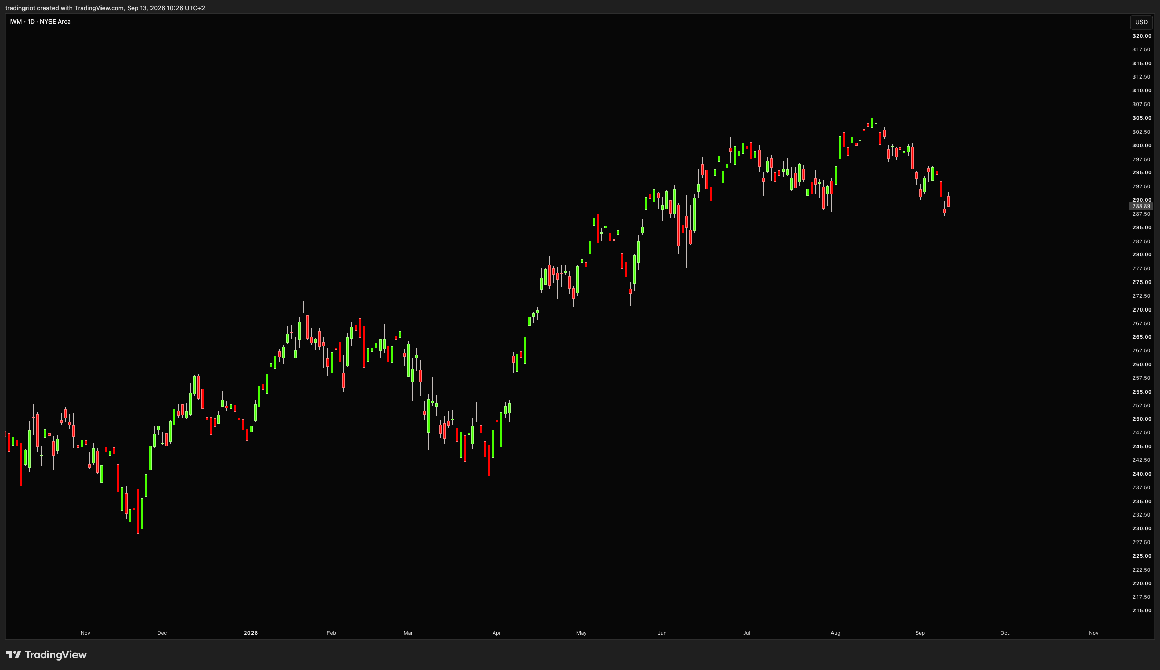
For IWM these two are pretty close, with mine being slightly more narrow, which makes sense since IWM has been fairly trendless lately.

You can find this model not only on the momentum page on the website for each optionable market, but it is also built straight into the position builder, where it is adjusted to the exact DTE.

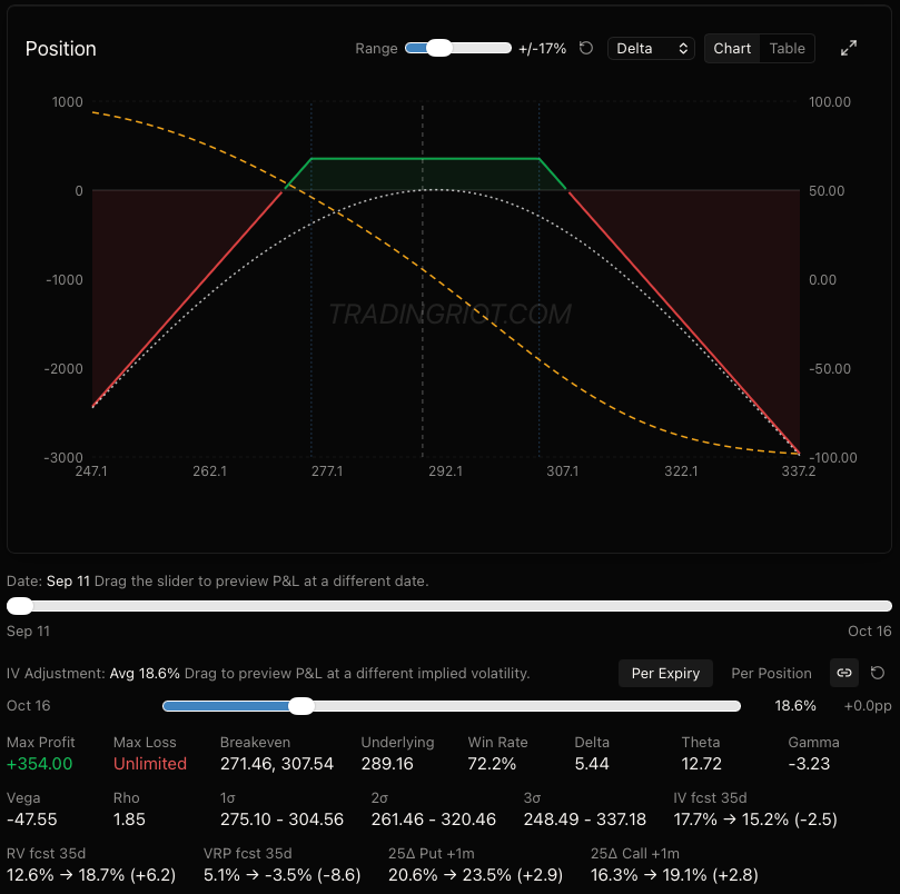
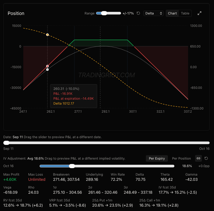
For IWM expiring in 35 days, 1 sigma moves based on my model are between 275 and 304.5 give or take, so I am selling the 275 put and 304 call. For this trade this put sits at 21 delta while the call is exactly at 16. You can also see that our delta starts very slightly positive, so we are better positioned for any positive drift.

Now for sizing, the backtest was sized to a 12.5% vol target while taking every single trade at a very fixed setting, so this is not really something we can do.

The first approach to sizing these trades, and arguably the more simple one, is trying to predict the worst-case scenario. Remember that we are using manual exit if term slope inverst so unless aliens are going to attack the earth tomorrow and everything opens at zero, we will exit trades ahead of a massive selloff like during the COVID or any other market stresses since term slope inverts fairly early on.

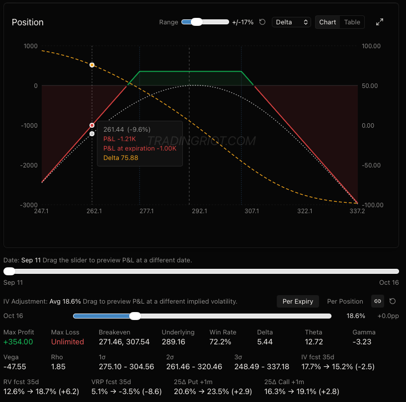
In the position builder, take a look at a two-sigma move and imagine the market closing there tomorrow; at that point term structure would be sure to be inverted, and you would see a signal to exit the trade. This should represent about 2-4% of your account, depending on how many positions you plan to open and how many positions in correlated markets you have opened.

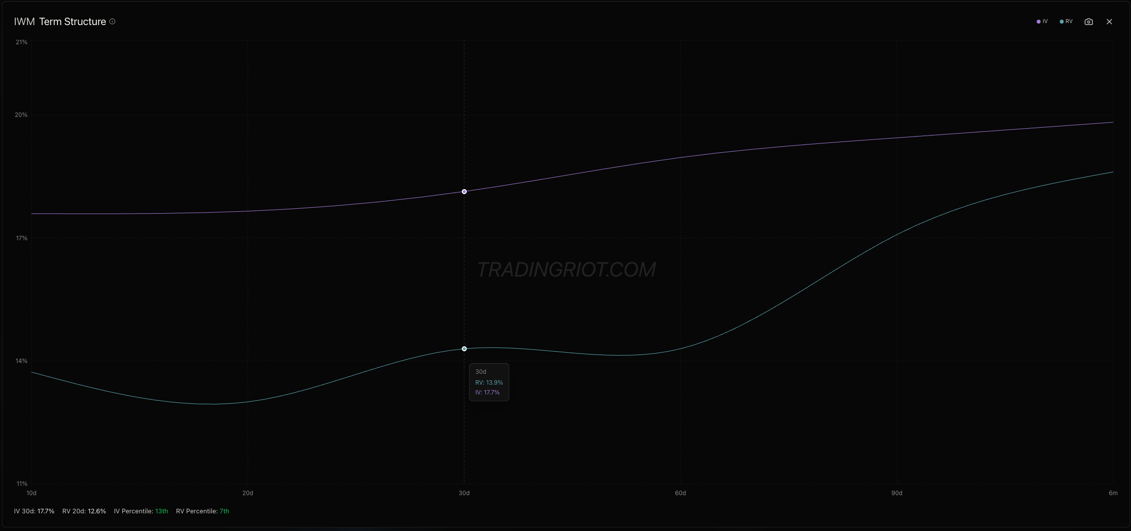
Another option is to simulate a realized volatility path. Going back to the analytics section, you can take a look at the term structure chart to see current IV and RV readings if you hover over the slope. Presently we are selling approximately 18% against 14% realized volatilty.

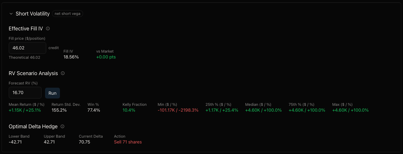
Under the position builder there is a short volatility block where you can import both of these numbers. Foremost, effective fill IV is essential; this represents the implied volatility based on your actual fill versus the market. I already spoke about the importance of the execution, but you should never overpay for these trades where your effective fill IV would be worse than the market.

Underneath you also enter the forecast realized volatility; if we put 14 there, it represents the current RV, the platform simulates 20,000 terminal prices at the inserted forecast realized volatility, prices them off your fill, and reports a Kelly fraction as mean return over its variance.

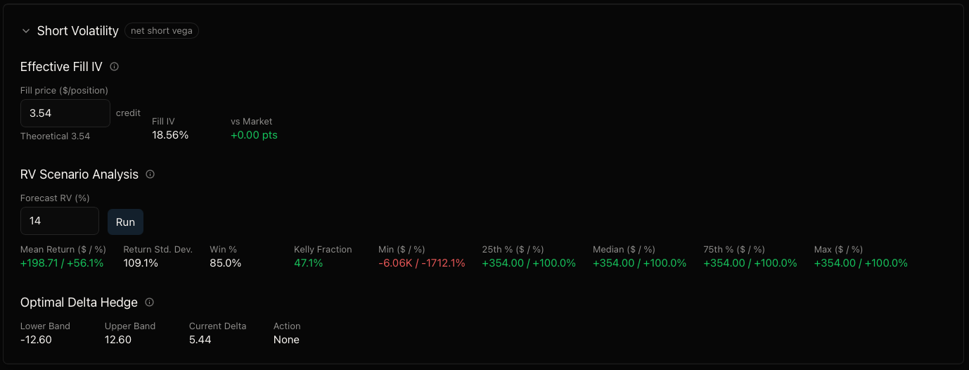
Kelly shows 47%; we are never going to use full Kelly, but rather a fractional number like 1/10th of the Kelly fraction. 4.7% in credit received is a lot, while realized volatility is very suppressed; this would mean at 1/10 Kelly on a $100,000 account, we are selling about 13 strangles, and if the market gaps tomorrow to that two-sigma move, we will lose approximately 15% of our account.

Back in the analytics section, you will find a volatility forecast window. Heterogeneous Autoregressive Volatility (HAR). The HAR model is a popular model for forecasting future realized volatility using, again, some very primitive mathematics:

𝑅⁢𝑉𝑡+1=𝛽0+𝛽1⁢𝑅⁢𝑉𝑑𝑡+𝛽2⁢𝑅⁢𝑉𝑤𝑡+𝛽3⁢𝑅⁢𝑉𝑚𝑡+𝑢𝑡+1

This article is already way too long for me to give any more in-depth explanation, and while the model is not perfect, it can be used as a good benchmark for future volatility since it also reports a confidence score.

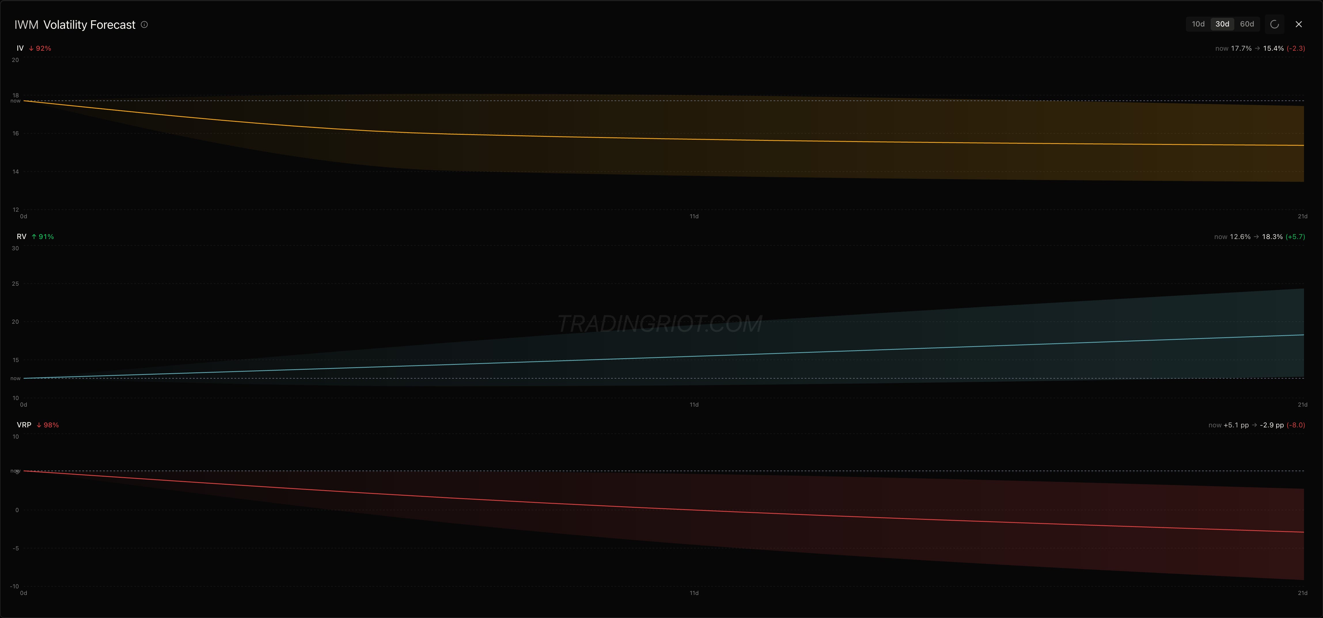
For IWM, you can see that the realized volatility over the next 30 days is actually expected to rise with about 91% confidence, and the forecast puts it at 18.3% with p10 at 12% and p90 at 24.5%.

The final number I put into forecast RV calculator varies based on what is IV thus VRP expected to do in upcoming 30 days as well.

In this case they are expected to fall, which can also be eyeballed on a long-term IV / RV chart that shows RV in historical lows.

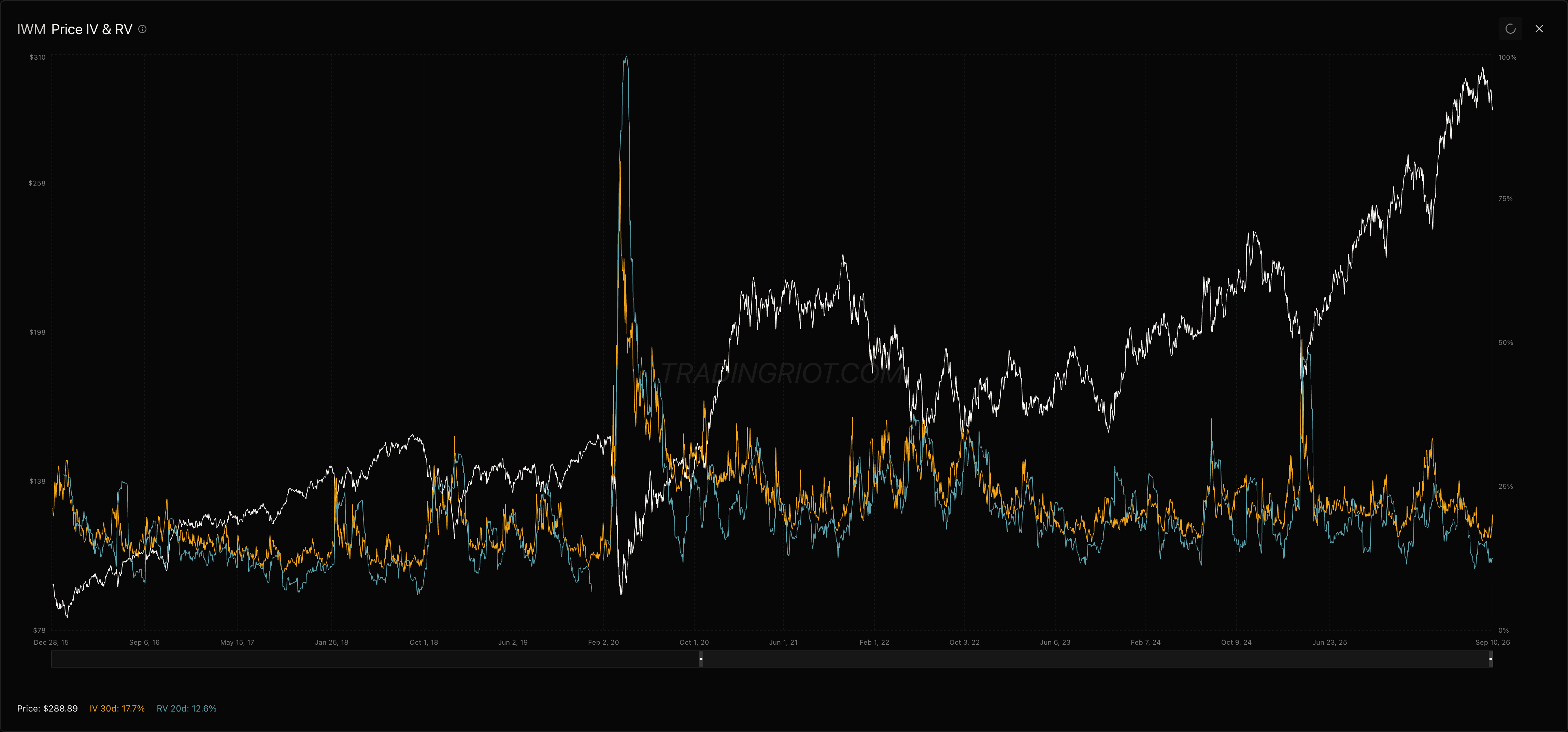
Because RV looks depressed and the model is showing high likelyhood of realized going up while implied going down, I will stick to 18.3% as my forecast realized volatility.

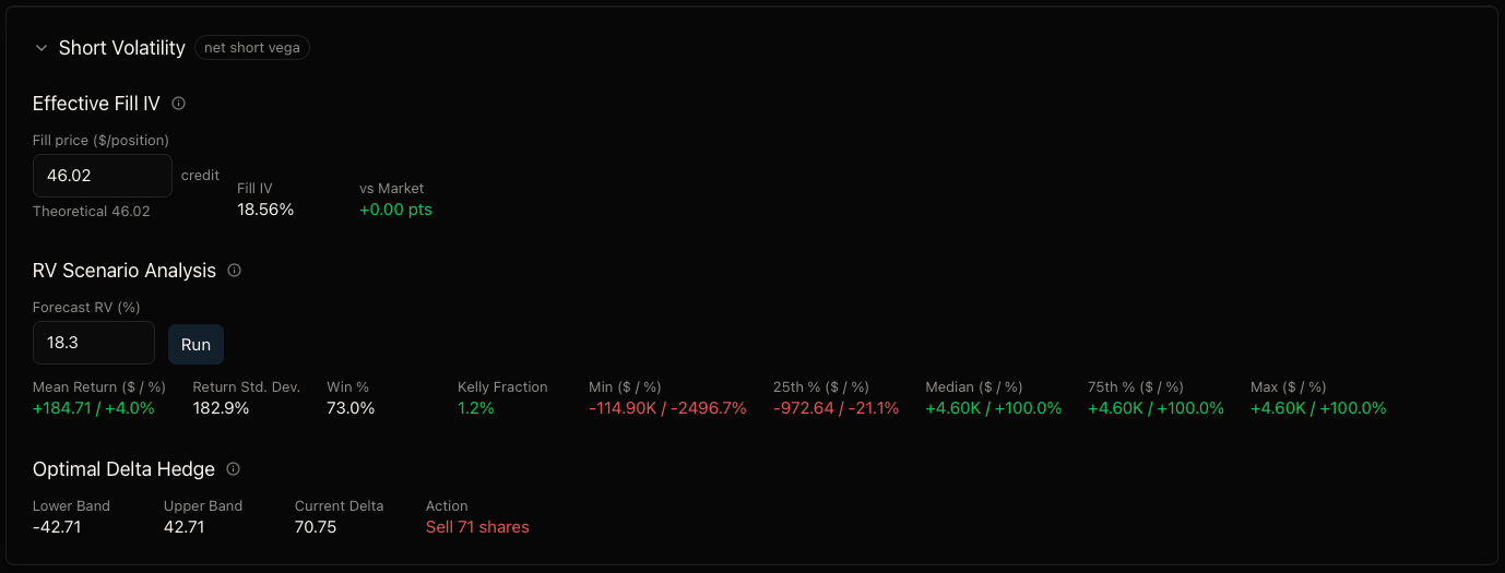
This 18.3% realized volatility is now on-par with current IV, and the Kelly Fraction dropped to 1.2%. Sticking to 1/10th of Kelly’s, is this telling us to risk $120 on a $100k account? That is not even one contract.

If you think about this, it makes sense. The current implied volatility at what we are getting filled at is 18.7%, and HAR forecast is telling us that in the next 30 days the volatility will be about 18.3%, so is this trade dead?

No, not really. Remember why we are trading this; we are trading this because markets often overstate the implied volatility for a plethora of reasons I have mentioned at the beginning of this article.

Going back to some testing, using about 10,000 historical measurements of ETFs when IV/RV > 1, the mean implied volatility overstated realized volatility by approximately 1.92 points.

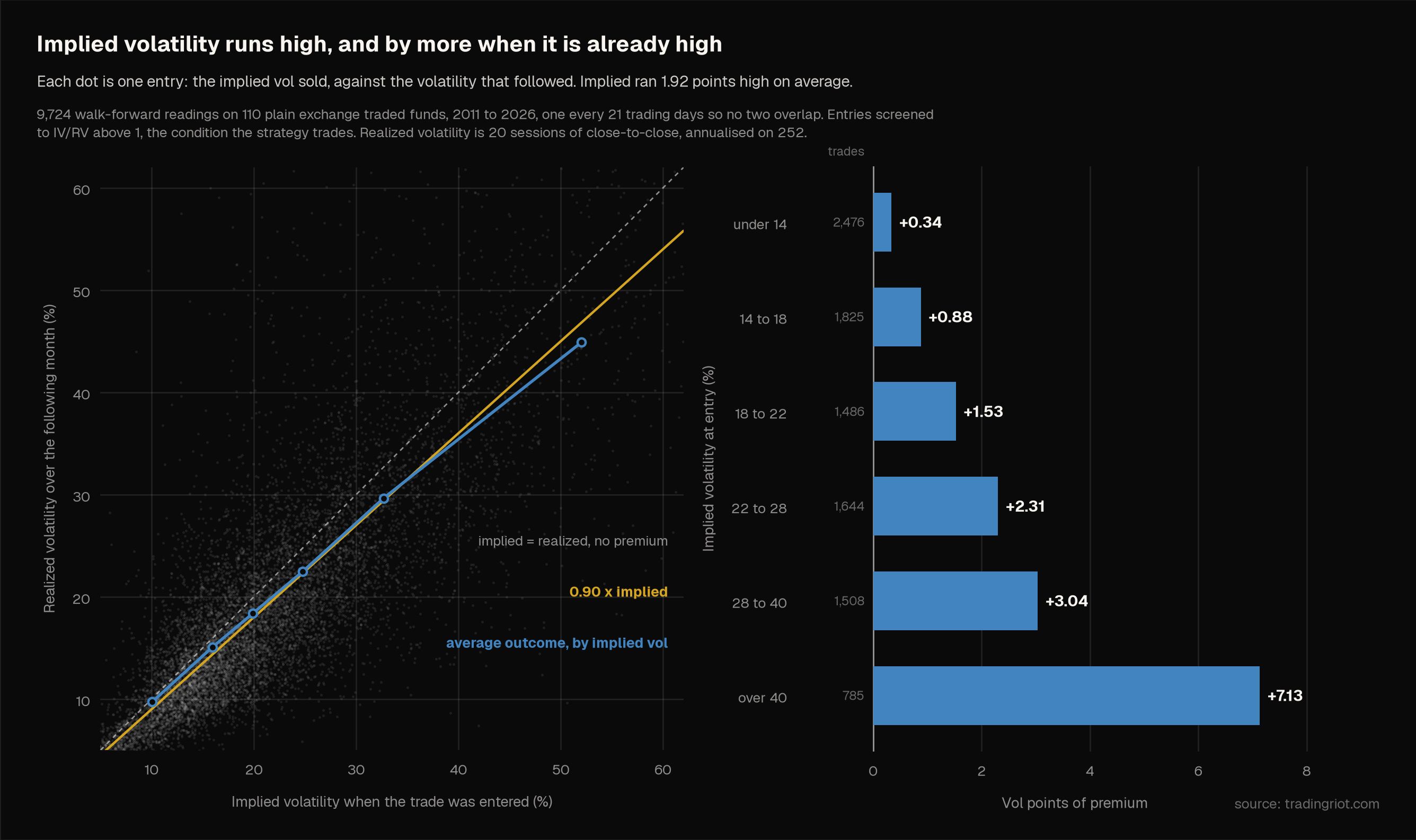
For that reason, you can calculate

fcstRV = 0.90 x fillIV

For this trade that turns out to be 10.4%, you are risking 1.04% per trade in credit received, and your loss on a two-sigma event tomorrow would be about 3.5%. If fcstRV from the HAR model were lower, you could use that number, but using multiplying your fill IV by 0.9 was well tested; therefore, you can use that while looking at the forecast from the HAR model as your volatility expectation.

After all is set and done, you should log your position and revisit it once per day. First and foremost, look at the term structure slope chart and see if it is inverted; if so, you will exit your trade (working your way out from bid to mid). The median holding period from the backtest was about a week, so you will be exiting many trades early, but this will also save you from end-of-the-world scenarios.

If you don’t think the world will end in the next month and you don’t fancy using the exit filter, you should at least delta hedge your trades. For that, use the delta hedging calculator on the website.

As proven by backtest, doing both doesn’t make sense, so just use one and stick to it. You will make more money by hedging but will also end up homeless in a COVID-like and probably some other scenarios like this February oil rally where an inverted curve would get you out right before the move, while delta hedging here probably wouldn’t help that much.

Conclusion

Short volatility strategies are not fun; you are accepting small payments in compensation for often account-wrecking risks.

If you are not careful, you can sell volatility for years and then give back everything and some within just a couple of days.

But as you could see in this article, by deploying a few clever and logical rules, we can turn this into a solid part of our portfolio, which doesn’t take much time to trade and track each day.

Two main things I would like you to take from this exercise are not trying to be a hero, especially if you are starting out with options, and making sure to start small and always be prepared to limit up or down.

Another thing is the execution: despite filtering for markets with liquid options and using only monthly contracts for expiration, options, especially at the wings, often lack liquidity. For anyone coming from the futures space, this can be a shock: how much each position needs to be worked and executed without overpaying. This strategy, like many others, can make or break based on the execution costs.