Everything You Should Know About Trading Options

Complete guide for options trading

Options are derivatives. That’s it. They derive their value from an underlying asset, just like futures or swaps.

There is no shortage of people who turn options knowledge into 4,000-word essays packed with third-order Greeks charts, volatility surfaces, and enough jargon to make it feel like rocket science.

While these obviously have their time and place, I do not assume you plan to become a quant or options market maker.

For retail traders, naming all third-order Greeks and calculating the theoretical fair value of an option using the Black-Scholes Model in your head is more telling about your social life than giving you any trading edge.

Contrary to popular belief, understanding how options work is not an edge. Understanding what product you trade should be the bare minimum.

But you still need to know the mechanics before you can do anything useful with them. This article covers all the fundamentals: what options actually are, how they’re priced, what drives their value, and most importantly, when it makes sense to buy them versus sell them.

By the end, you’ll have a complete picture of how options trading works and enough context to start thinking about where real edges might exist.

Before we dive into the article, if you want analytics for over 1,000 markets across options, crypto, and futures while learning systematic trading strategies that harvest different risk premiums across multiple asset classes, check out tradingriot.com. Use code “ANALYTICS” for 50% off your first month.

What Is an Options Contract?

Before we go into any complex stuff, I figured it would be nice to give you an example outside of financial markets that completely covers options basics and Greeks.

Options give the holder the right, but not the obligation, to buy or sell the underlying asset at a specified price on a specified date.

The buyer of the option pays a premium. The seller of the option receives the premium.

To translate this into much simpler terms, let’s say you want to buy a house and find a seller.

You ask the seller if he can issue you an option that expires in 12 months and gives you the right to buy the house for $500,000. He will also receive a premium for this option, which equals $10,000.

If he agrees, you have the right to buy the house for $500,000 anytime in those twelve months, and you don’t need to care about housing market price fluctuations.

Let’s say the twelve months passed, and the current price of the house is only $450,000.

In this case, you are obviously not going to buy the house for 500k, so you will not exercise your right to buy it.

But you lost the $10,000 premium, which was the risk you put up.

In another example, let’s say that the housing market skyrocketed, and the current price of that house is now $700,000.

Of course, you are going to exercise your right to buy the house for $500,000, and you made a profit of $190,000 (final price (700k) - strike price (500k) - premium (10k)).

Let’s now flip the table and look at the situation from the perspective of the option seller.

In the first scenario, the option expired worthless as the price of the house was below the option price, and the seller ended up with the premium he was paid.

In the second scenario, the option ended up in the money, and the seller technically lost $190,000 as he now has to sell a house that has a $700,000 value for only $500,000 (minus the premium).

This principle is the same in options trading.

• If you are an option buyer, your risk is limited only to the premium paid, and your reward is technically unlimited.

• If you are an option seller, your reward is limited only to the premium you receive, and your risk is technically unlimited.

Although this might seem like selling options is pure stupid, you will find out than more often than not options selling is actually preferred, one of the cases was already covered in trading options around earnings.

What makes options complicated is that several factors influence the price of the option during those twelve months.

The most obvious factor is the price of the house itself. If the house goes up in value, your option to buy it at $500,000 becomes more valuable. If it drops, your option loses value.

But price isn’t the only thing at play. Time works against you as the option buyer. You paid $10,000 for twelve months of optionality, and every day that passes, a piece of that value disappears. Even if the house price doesn’t move at all, your option is worth less tomorrow than it is today.

Uncertainty also plays a role. If a rumor spreads that a tech company might build nearby, the house could go to $800,000 or crash to $400,000. That uncertainty alone makes your option more valuable, even without any actual price movement.

Interest rates matter too. For shorter-dated options, the impact is negligible, but for longer-dated ones or in fast-moving rate environments, it starts to add up.

All of these factors act on your option at the same time. On any given day, the house price might go up, but time passed and uncertainty dropped. The price you see is the net result of all these forces pulling in different directions, and they work opposite for option buyers and sellers. We will cover each of these in detail later in the article.

Options Basics

So now that you know how options work, it is a great time to translate this knowledge into the markets.

Although the example of buying a house was rather simple, if you open an option chain, it looks like everything but simple.

Reading an Options Chain

When you want to open an order on futures, it is usually very straightforward. You either buy or sell.

On options chains, there are many more elements to consider.

Calls and Puts

There are two types of options contracts: calls and puts.

A call option gives you the right to buy the underlying asset at the strike price. You buy calls when you think the price is going up.

A put option gives you the right to sell the underlying asset at the strike price. You buy puts when you think the price is going down.

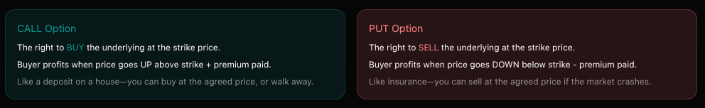
Worth to keep in mind that this is slightly different from futures where you go long or short, in options buying a put is still speculating that price will go down despite you are buyer of options contract.

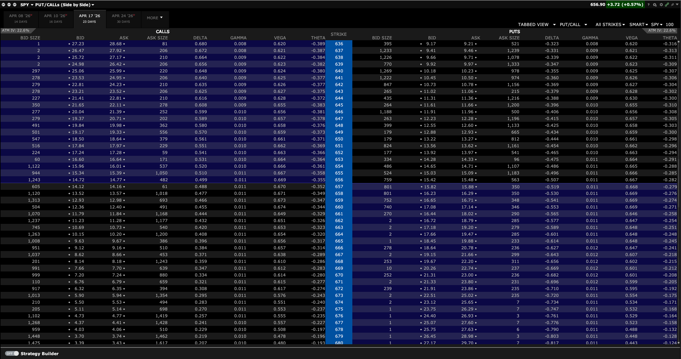
Looking at our SPY options chain, you’ll notice calls on the left side and puts on the right side, with strike prices running down the middle. This is the standard layout across most platforms.

Both sides of the chain work the same way mechanically. They have the same columns: bid, ask, delta, gamma, vega, theta. The difference is the directional bet. Calls profit when SPY goes up. Puts profit when SPY goes down.

Strike Price and Moneyness

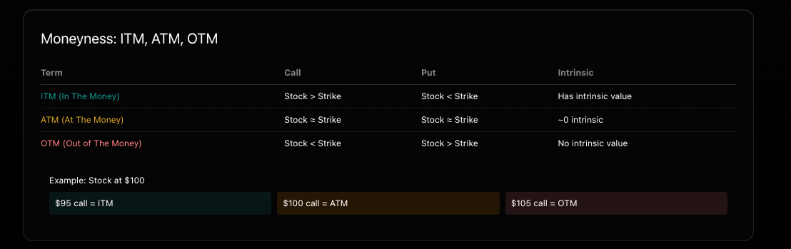
The first thing you need to pick is a strike price. When choosing one, you’ll come across three terms that describe the relationship between the strike and the current price of the underlying asset. This relationship is called the “moneyness” of the option.

Looking at our SPY options chain with SPY trading at $657.44:

• In the money (ITM): the option has intrinsic value. For calls, this means the strike is below the current price. The 640 strike call is in the money because you’d have the right to buy SPY $17.44 below where it currently trades. For puts, it’s the opposite. The 670 strike put is in the money because you’d have the right to sell SPY $12.56 above where it currently trades.

• At the money (ATM): the option strike is closest to the current price of the underlying. The 657 strike is the nearest at-the-money option in our chain, for both calls and puts.

• Out of the money (OTM): the option has no intrinsic value. The 670 strike call is out of the money because SPY would need to rally above $670 before that call has any value at expiration. The 640 strike put is out of the money because SPY would need to drop below $640 for that put to have value at expiration.

Notice that what counts as ITM for calls is OTM for puts, and vice versa. The 640 strike call is in the money, but the 640 strike put is out of the money. Same strike, opposite moneyness.

Intrinsic and Extrinsic Value

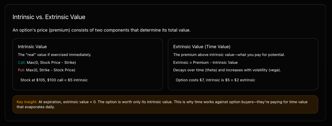
Every option premium consists of two components: intrinsic value and extrinsic value.

Intrinsic value is the real, tangible value of the option if it were exercised right now.

For calls: intrinsic value = underlying price - strike price (or zero, whichever is higher). For puts: intrinsic value = strike price - underlying price (or zero, whichever is higher).

The 640 strike call on SPY at $657.44 has an intrinsic value of $17.44. The 670 strike call has zero intrinsic value because SPY hasn’t reached that level yet. On the put side, the 670 strike put has $12.56 of intrinsic value, while the 640 strike put has none.

Extrinsic value is everything else baked into the premium on top of intrinsic value. It depends on time to expiration, volatility, dividends, and the risk-free interest rate.

If we compare two options with the same strike, one expiring next week and one expiring a month from now, the longer-dated option will have a higher extrinsic value (they are more expensive). More time means more opportunity for the underlying to move, and that optionality costs money.

At expiration, extrinsic value is always zero. The option is worth only its intrinsic value. This is why time works against option buyers. Every day, a piece of that extrinsic value evaporates.

Premium

The premium is what the option costs. Looking at our chain, the 657 strike call (closest to at the money) shows a bid of $13.52 and an ask of $13.57.

The bid is the highest price a buyer is willing to pay. The ask is the lowest price a seller is willing to accept. If you want to buy this call immediately, you pay the ask price of $13.57. Since SPY options have a contract multiplier of 100, your actual cost is $13.57 x 100 = $1,357 per contract.

The contract multiplier applies to most equity and ETF options. When you see a premium quoted as $13.57, that’s the per-share price. One contract controls 100 shares, so you always multiply by 100 to get the real dollar amount.

The difference between the bid and the ask is called the spread. On this 657 strike call, the spread is $0.05 ($13.57 - $13.52). That spread is a cost to you. The moment you buy at the ask for $13.57, you could only sell at the bid for $13.52, meaning you’re immediately down $0.05 per share, or $5 per contract.

Spreads vary across the chain. At-the-money options with high volume tend to have tight spreads, like the $0.05 we see here. Deep out-of-the-money options with less liquidity will often have much wider spreads. That wider spread is a hidden cost that eats into your potential profit, and it’s something many new options traders overlook.

Expiration and Exercise Style

Every option has an expiration date. In our chain, we can see multiple expirations available: April 8th (14 days), April 10th (16 days), April 17th (23 days), and April 24th (30 days). This is the date by which the option either has value or expires worthless.

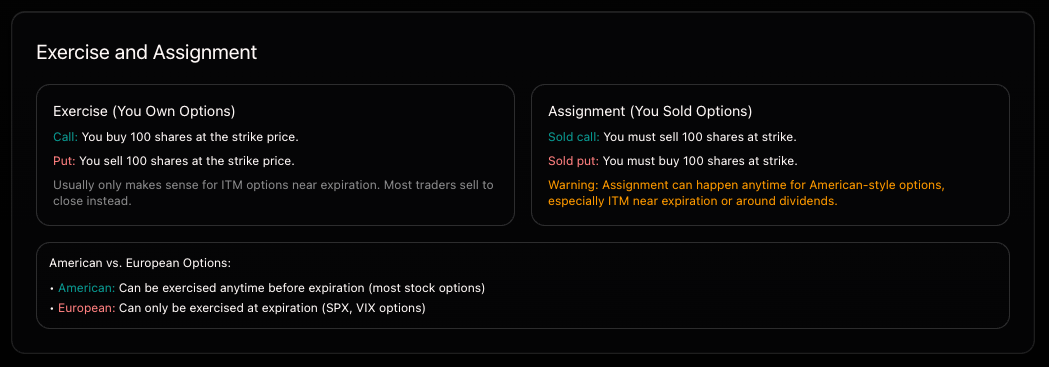
There are two styles of options when it comes to how they can be exercised.

American-style options can be exercised at any point before expiration. Most equity and ETF options, including SPY options, are American-style.

European-style options can only be exercised at expiration. It doesn’t matter if the underlying moves in your favor during the life of the option. You have to wait until the expiration date. Most index options, like those on SPX, are European-style.

Exercise and Assignment

When you own an option and decide to use your right, that’s called exercising.

If you exercise a call, you buy 100 shares of the underlying at the strike price. If you exercise a put, you sell 100 shares at the strike price.

Most traders never exercise their options. They simply sell the option back to close the position and collect the profit. Exercising usually makes less money because you throw away any remaining extrinsic value. If your 640 call is worth $18.50 but only has $17.44 of intrinsic value, selling it gets you the full $18.50. Exercising only captures the $17.44.

The exception is deep in-the-money options very close to expiration, where extrinsic value is basically zero. In that case, exercise and selling are roughly the same.

Now here’s where it gets important if you’re an option seller. Assignment is the other side of exercise. When someone exercises their option, a seller on the other side gets assigned.

If you sold a call and get assigned, you must sell 100 shares at the strike price. If SPY is at $680 and you sold the 660 call, you’re selling shares at $660 regardless of the market price. If you don’t already own the shares, your broker buys them at $680 and sells them at $660, and that $20 per share loss (minus the premium you collected) is yours.

If you sold a put and get assigned, you must buy 100 shares at the strike price. If SPY dropped to $620 and you sold the 650 put, you’re buying shares at $650 when they’re worth $620. That’s a $30 per share loss, minus the premium.

For American-style options, assignment can happen at any time, not just at expiration. It’s most likely to happen when the option is deep in the money and has very little extrinsic value remaining, or right before an ex-dividend date. If you sold an in-the-money call on a stock that’s about to pay a dividend, the option holder might exercise early to capture that dividend, and you’ll wake up to an assignment notice.

This is why many option sellers prefer to trade European-style index options like SPX. No early assignment risk.

Put-Call Parity

There is a fundamental relationship between the prices of calls and puts at the same strike and expiration. This is called put-call parity, and the basic formula is:

Call + Strike = Put + Stock Price

Or rearranged: Call - Put = Stock Price - Strike

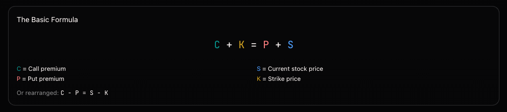
This means if you know three of the four values, you can calculate the fourth. More importantly, it tells you that calls and puts at the same strike always carry the same amount of extrinsic (time) value.

Let’s use our SPY chain to check this. SPY is at $657.44, and we’ll look at the 657 strike.

The 657 call mid-price is roughly $13.54 (averaging bid $13.52 and ask $13.57). The 657 put mid-price is roughly $13.20 (averaging bid $13.03 and ask $13.38).

Call - Put = $13.54 - $13.20 = $0.34 Stock - Strike = $657.44 - $657 = $0.44

These numbers are close but not identical. The small difference comes from interest rates, expected dividends, and the bid-ask spread. In textbook conditions, they’d match perfectly. In real markets, they’re always very close, and when they drift apart, market makers jump on the arbitrage and push them back in line.

Why does this matter for you? A couple of reasons.

First, it tells you that calls and puts are not independent instruments. They’re mathematically linked. You can’t have a situation where calls are “cheap” and puts are “expensive” at the same strike without someone arbitraging that away.

Second, it means you can create synthetic positions. Buying a call and selling a put at the same strike is synthetically the same as owning the stock. Buying a put and selling a call is the same as being short. This becomes useful when building more complex strategies.

Third, it’s a quick sanity check. If you’re looking at option prices and something feels off, run the parity formula. If the numbers don’t line up within a reasonable margin, something is wrong with the quotes, or there’s a dividend or hard-to-borrow situation affecting pricing.

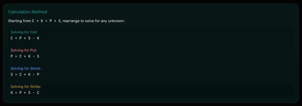
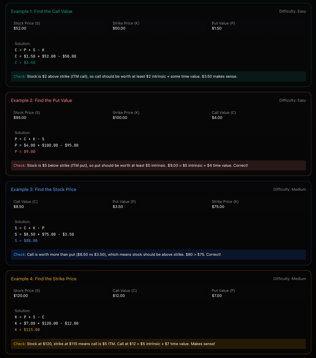
Below are few examples on calculating put/call parity, just a small note In real markets, you may see a Rev/Con adjustment added to the formula. This accounts for ,Interest rates, dividends and borrow costs.

For learning purposes, we’ll use the basic formula. Rev/Con is typically small (a few cents to a dollar) and professionals use it for arbitrage calculations.

The Greeks

Now for the scary stuff: option Greeks. As I mentioned, Greeks represent variables that determine the option’s price, which is constantly changing.

There are first, second, and third-order Greeks.

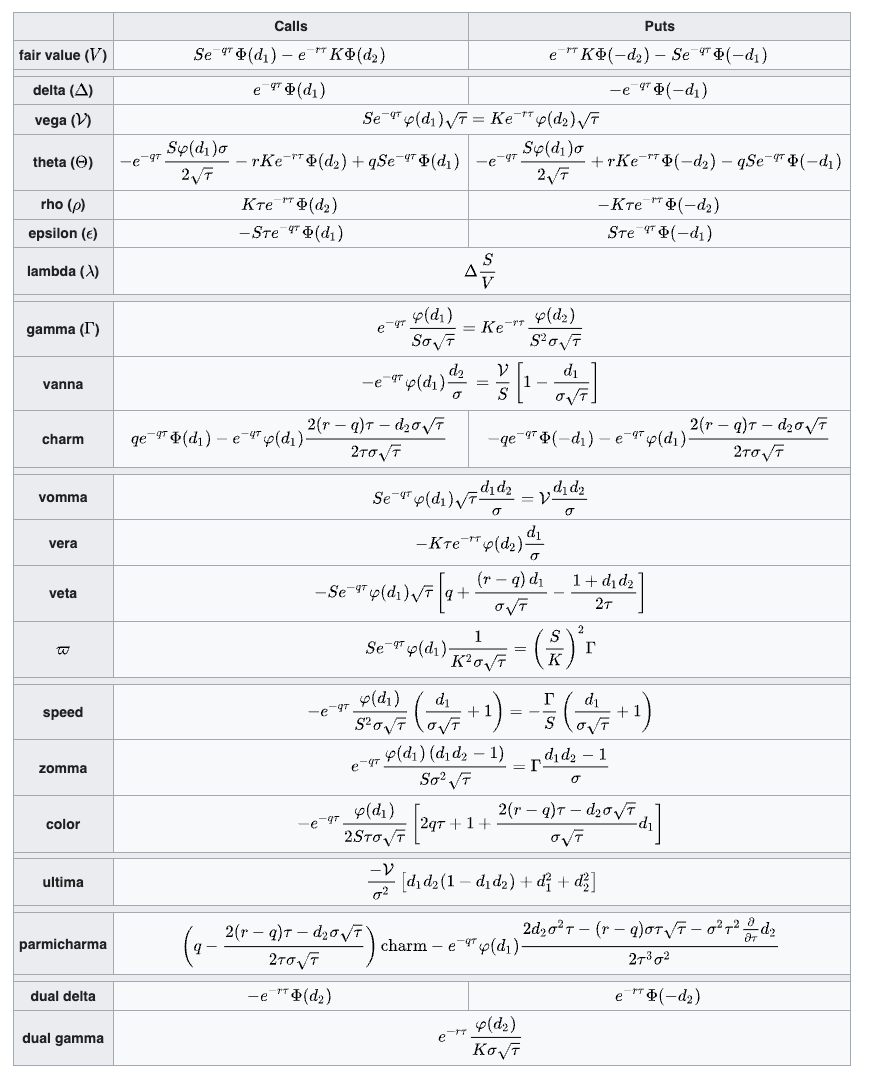
If the image above looks insane to you, don’t worry. In reality, you only need to understand first-order Greeks (second-order are useful for day trading), and the math is really not important.

In my trading, I refuse to acknowledge things such as parmicharma, which sounds like Italian ham, or speed, that is solely reserved for 3am on a weekend when you want the night to keep going.

The Black-Scholes Model

The Black-Scholes Model (BSM) from 1973 is the foundation of modern options pricing. It provides a theoretical price for European options and serves as the basis for calculating the Greeks. No model perfectly captures reality, but Black-Scholes gives us a common language for pricing options. You don’t really need to know the formula since everything is calculated for you inside your broker, but it’s still a good exercise to understand what’s happening under the hood.

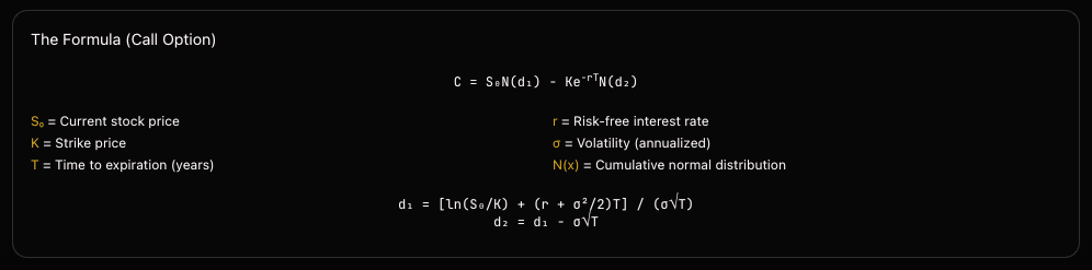
If this still looks scary, forget the math for a moment. Black-Scholes answers one question: “What should I pay for the right to buy a stock at a fixed price in the future?”

It does this in four steps.

First, start with intrinsic value. If the stock is at $105 and the strike is $100, there’s $5 of real value baked in.

Second, add time value. More time means more chance for the price to move in your favor. An option can be worth something even if it’s currently out of the money, simply because there’s still time left.

Third, figure out how much that time value should be. This is where volatility comes in. Higher volatility means bigger potential moves, which means more time value. Volatility is the single most important input in the model.

Fourth, discount for the time value of money. You’re paying now for something that settles later, so the model adjusts for interest rates.

The Greeks are just partial derivatives of this formula. Each Greek tells you how the option price changes when one of these inputs moves.

Black-Scholes makes several assumptions that don’t hold up perfectly in the real world.

It assumes volatility stays constant. In reality, volatility changes all the time. It assumes stock returns follow a log-normal distribution. In reality, markets have fat tails, meaning crashes happen more often than the model expects. It assumes no dividends, though adjusted versions exist for stocks that pay them. It assumes European-style exercise only, while most stock options are actually American-style.

Despite all of this, Black-Scholes remains the standard. When you hear “implied volatility,” that’s the volatility value that, when plugged into the Black-Scholes formula, produces the current market price. Implied volatility isn’t directly observable. It’s backed out from the model. The entire options market speaks in volatility terms because of this framework.

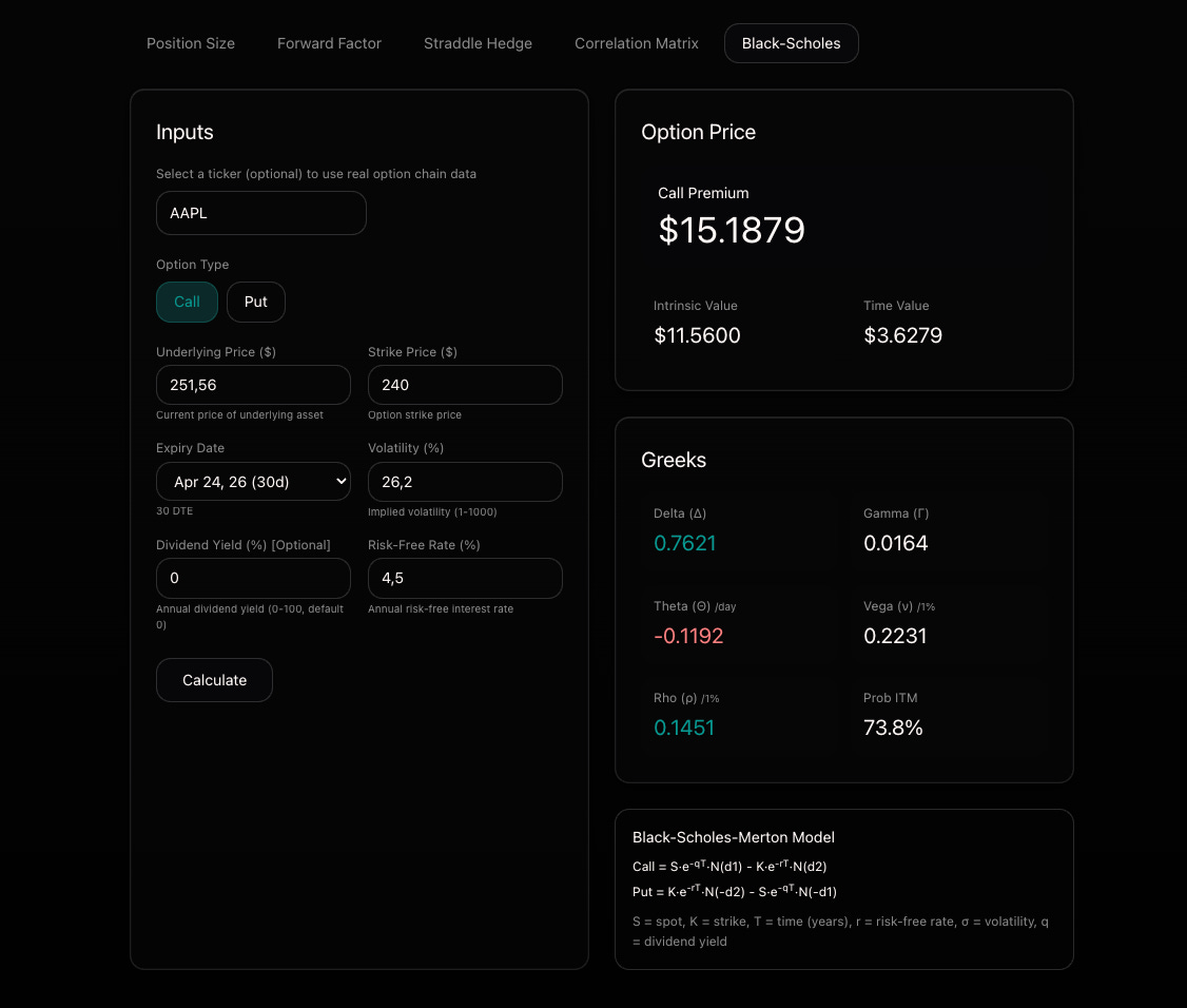
You will find free calculators on tradingriot.com, with a BSM calculator included, so you can see how the calculation works across a range of different options.

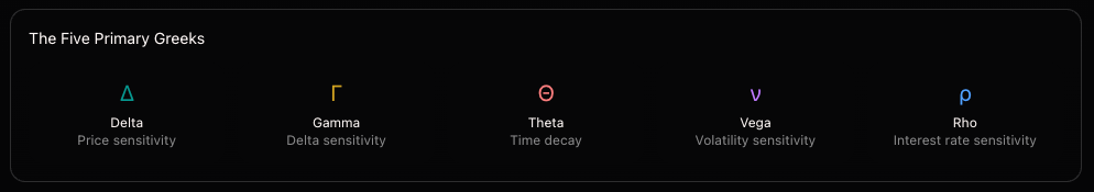
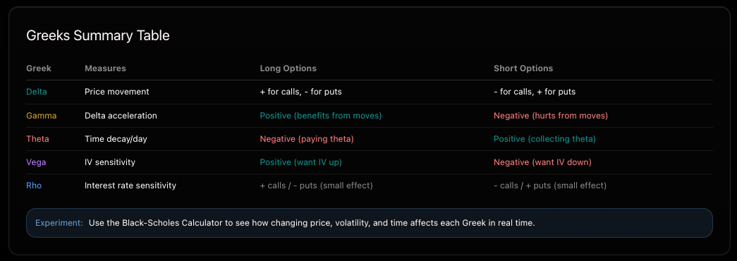
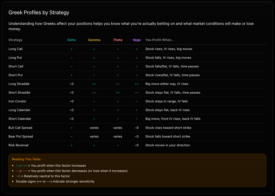
Five Primary Greeks

There are five Greeks you will care about: Delta, Gamma, Theta, Vega, and Rho.

These are often called first-order Greeks, although fun fact (not really) is that Gamma is actually a second-order Greek of Delta.

The Greeks measure how an option’s price changes relative to various factors. Understanding them is essential for managing risk and knowing what you’re actually betting on.

Delta

Delta measures how much an option’s price moves for a $1 change in the underlying. It ranges from 0 to 1 for calls and 0 to -1 for puts.

A deep in-the-money call has a delta close to 1.00, meaning it moves almost dollar for dollar with the stock. An at-the-money call sits around 0.50. A far out-of-the-money call might have a delta of 0.05, barely reacting to price changes at all. Puts work the same way but in reverse, with negative deltas.

Let’s say the stock is at $100 and you own a $100 call with a delta of 0.50. If the stock moves to $101, your call gains roughly $0.50. If the stock drops to $99, your call loses roughly $0.50.

Delta also has two practical interpretations beyond price sensitivity. First, it roughly approximates the probability of the option expiring in the money. A delta of 0.50 means roughly a 50% chance. This is less accurate the further out in time you go, more on that maybe sometimes in future. Second, it tells you your equivalent share exposure. One contract with a 0.50 delta gives you exposure equivalent to holding about 50 shares.

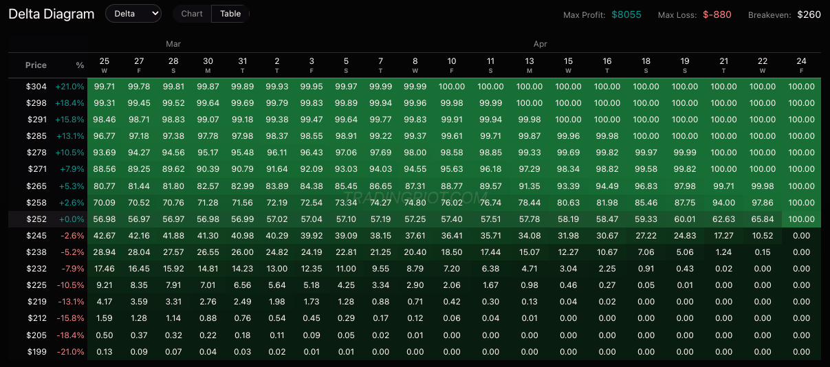
Above you can see a delta diagram for a long call. The more in the money your call is, the closer to 1.00 delta it gets. Once an option reaches a delta of 1.00, the position behaves the same as owning 100 shares of the underlying.

Position builder is free to use on tradingriot.com.

Gamma

Gamma measures how fast delta changes as the underlying moves. Think of delta as speed and gamma as acceleration.

At-the-money options have the highest gamma. Their delta is the most sensitive to price changes. Deep in-the-money and far out-of-the-money options have low gamma because their deltas are already close to their extremes and don’t move much.

Here’s a quick example. You hold an ATM call with a delta of 0.50 and gamma of 0.05. The stock moves up $1, and your delta increases to roughly 0.55. Another $1 up and it’s around 0.60. Your position gets increasingly bullish as the stock rises.

Gamma gets particularly intense near expiration for at-the-money options. With days left, a small move in the stock can flip delta from 0.30 to 0.70 in a hurry. This is why expiration week can feel chaotic, you can see how on Gamma diagram the highest gamma is ATM right before the expiration.

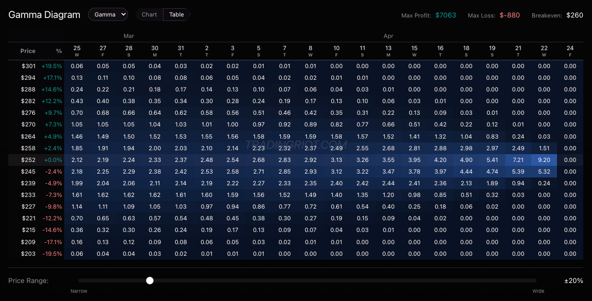
If you’re long options, gamma works in your favor. Your delta adjusts to catch profitable moves in either direction. If you’re short options, gamma works against you. The more the stock moves, the worse your position gets. This long gamma vs. short gamma dynamic is one of the most important concepts in options trading, and we’ll revisit it when we talk about strategies.

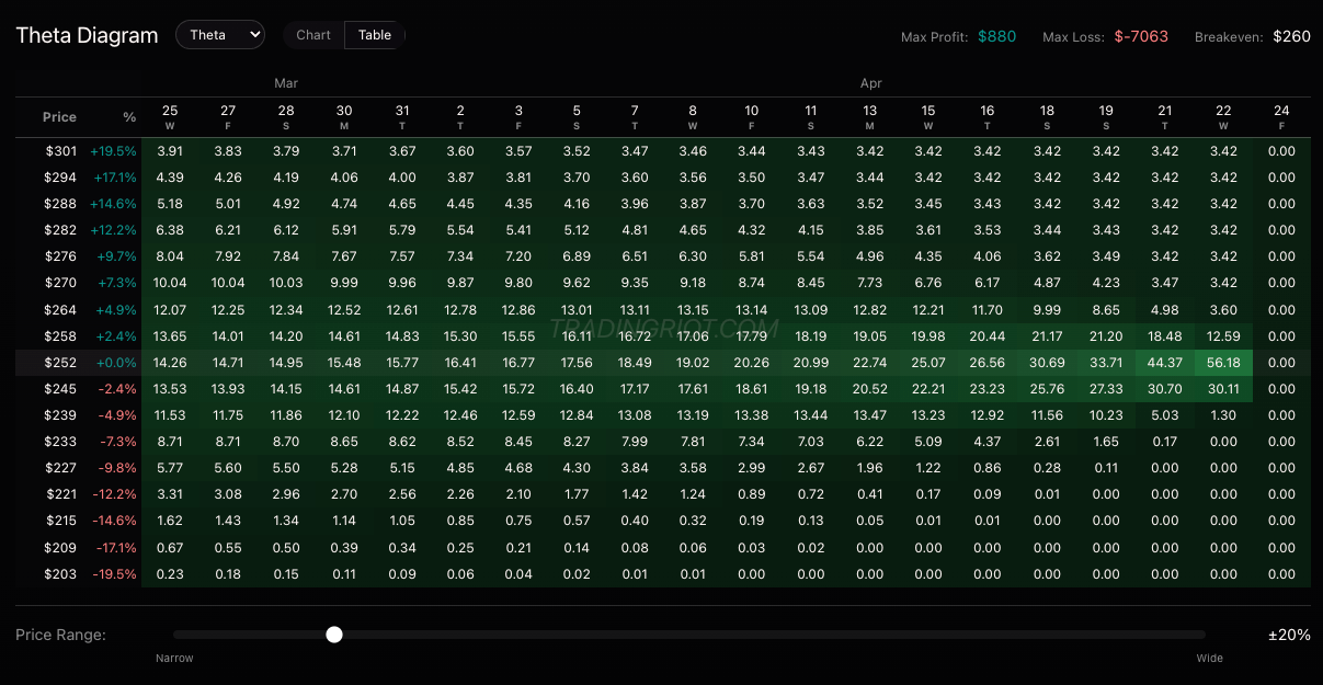
Theta

Theta measures how much value an option loses each day, all else being equal. It’s expressed as a negative number for option buyers because time is always working against you.

At-the-money options have the highest theta. They carry the most extrinsic value, so they have the most to lose. Deep in-the-money and far out-of-the-money options have lower theta because there’s less extrinsic value to decay.

Take an ATM call priced at $3.00 with a theta of -$0.08. If nothing changes overnight, that option is worth roughly $2.92 tomorrow. After five days of nothing happening, it’s down to about $2.60. You lost $0.40 just by holding it.

Theta decay is not linear. Early in the option’s life, decay is slow. You barely notice it. As expiration approaches, it accelerates. The last two weeks are where theta really starts to bite. This is why short-dated options lose value so fast and why option sellers love selling with 30 to 45 days left, capturing the steepest part of the decay curve.

Theta for long call

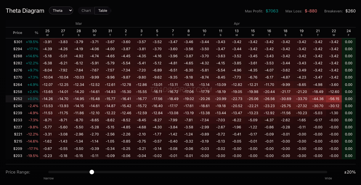
The key insight: theta is the cost of holding long options and the profit of holding short options. Option sellers make money from time passing. Option buyers lose it.

Theta for short call

Vega

Vega measures how much an option’s price changes for a 1% change in implied volatility. This is where options get interesting, because when you trade options, you’re often betting on volatility rather than direction.

At-the-money options have the highest vega. Longer-dated options have higher vega than shorter-dated ones because there’s more time for volatility to play out. All options have positive vega, meaning higher implied volatility increases every option’s price.

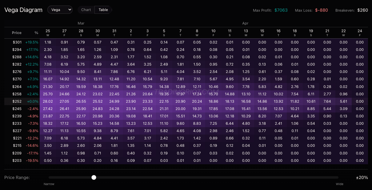
Here’s an example. You own an option priced at $5.00 with a vega of 0.15. Implied volatility rises from 25% to 26%, and your option goes to $5.15. If implied volatility drops from 25% to 20%, your option falls to $4.25. That’s a $0.75 loss from a volatility move alone, with the stock potentially not having moved at all.

This is why you can buy a call, have the stock go up, and still lose money. If implied volatility got crushed at the same time, the vega loss can outweigh the delta gain. It happens all the time around events like earnings, where implied volatility collapses after the announcement regardless of which direction the stock moves.

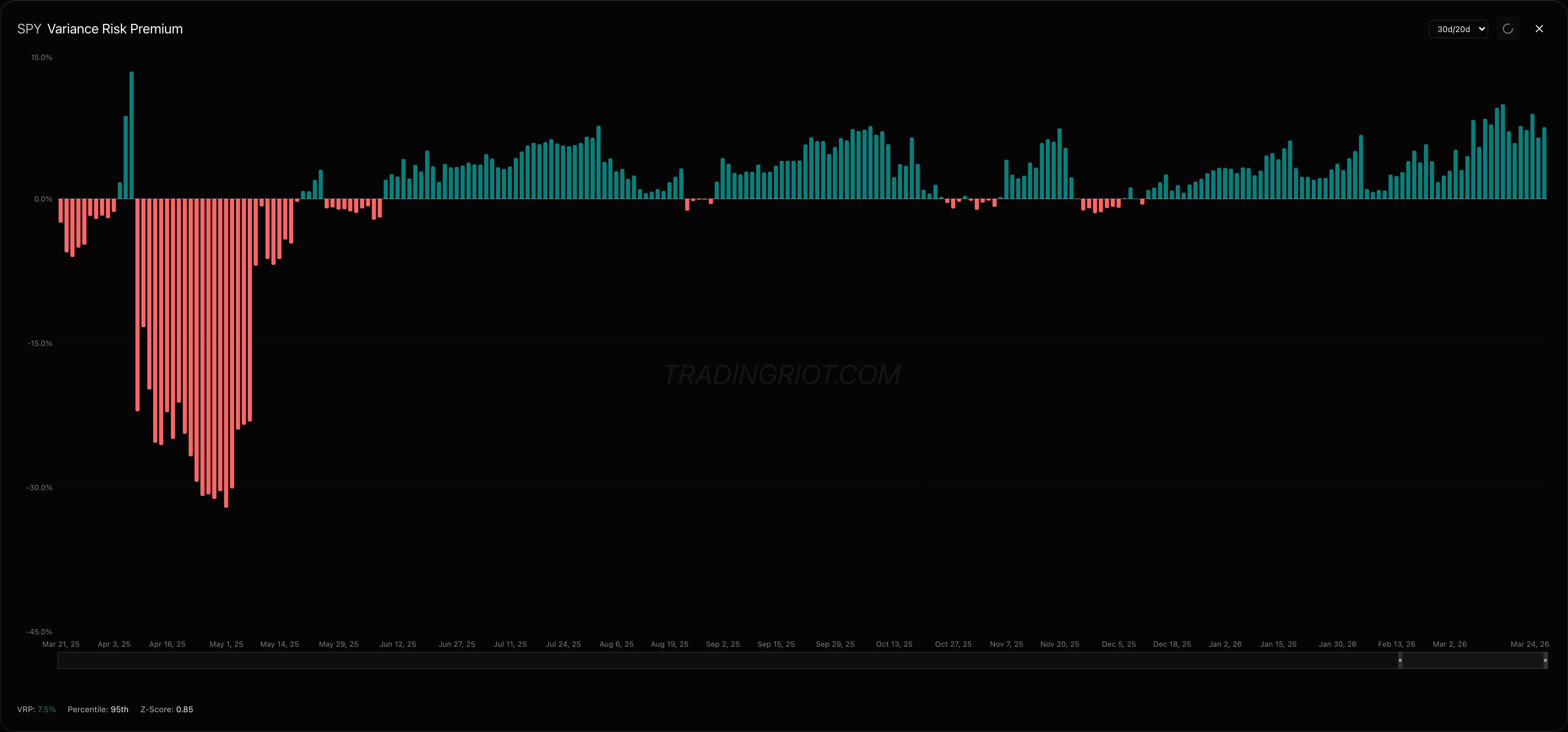
Understanding vega is what separates directional gamblers from actual options traders. Strategies like the variance risk premium, which we cover extensively on TradingRiot, exist specifically to exploit the tendency of implied volatility to overstate realized volatility. You’re selling high vega when IV is elevated and collecting the difference.

Rho

Rho measures how much an option’s price changes for a 1% change in interest rates. For most traders, it’s the least relevant Greek because interest rates move slowly and predictably compared to price and volatility.

Calls have positive rho, meaning higher rates make calls more valuable. Puts have negative rho, so higher rates make puts less valuable. Longer-dated options have higher rho because there’s more time for rates to matter.

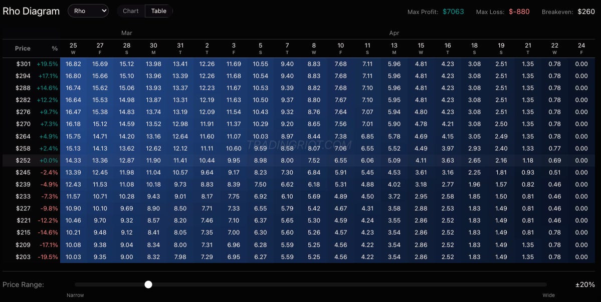
For a LEAPS call with a one-year expiration and a rho of 0.25, a 1% rate increase adds about $0.25 to the option’s price. For a 30-day option, rho might be 0.02, which is basically nothing.

Rho starts to matter in a few specific situations: LEAPS options with a year or more to expiration, deep in-the-money options where you’re essentially financing a stock purchase, and high-rate environments or periods around Fed decisions. For short-term weekly or monthly options, you can safely ignore rho. Delta, gamma, theta, and vega will dominate your P&L.

Second and Third Order Greeks

Second-order Greeks measure how the primary Greeks change with respect to price, time, and volatility. Third-order Greeks measure how second-order Greeks change. These are the “Greeks of Greeks,” and they’re used primarily by market makers managing large books and systematic funds running precise hedging.

For most retail traders, you can safely ignore the majority of them. Understanding delta, gamma, theta, and vega covers 95% of what you need for informed trading decisions.

That said, two second-order Greeks are worth knowing about if you trade short-dated options.

Vanna measures how delta changes when IV changes, or equivalently, how vega changes when price moves. This matters because when price falls and IV rises simultaneously, vanna effects amplify the move. Market makers who are short options get hit on both sides at once, forcing aggressive hedging that pushes the market even further. This is the dealer hedging amplification effect you hear about during sharp selloffs. On 0DTE options, vanna can cause wild delta swings. A small move in the underlying combined with an IV spike can flip a position from barely directional to heavily exposed in minutes.

Charm measures how delta changes as time passes. OTM options lose delta over time while ITM options gain delta, even without any price movement. Dealers have to rehedge daily to account for this drift. In 0DTE trading, charm is on overdrive. With the entire time decay compressed into a single session, delta shifts rapidly throughout the day. A slightly OTM call at the open can see its delta melt away by lunch even if price hasn’t moved, and the dealer hedging flows created by this process contribute to the intraday pinning effects you see around large open interest strikes.

Everything beyond vanna and charm, things like vomma, speed, color, zomma, or ultima, is firmly in market maker and quant territory. Interesting to know they exist, but not something you need to lose sleep over.

Volatility

If you have made it this far in the article, you might be asking yourself a very simple and logical question, which most likely goes something like: “Why would I bother with all of this when I can just trade futures?”

That’s understandable. While there is definitely a use case for buying options as directional bets since they can have highly convex payouts and offer great risk-to-reward ratios, the truth is they often bring a large amount of complexity. You’re watching Greeks, timing entries, and racing against theta bleeding out your debit the entire time.

One of the main reasons for choosing options over other derivatives is being able to speculate on volatility.

What Is Volatility?

Volatility measures how much an asset’s price wiggles. High volatility means wiggles a lot. Low volatility means calm, steady movement.

In statistical terms, volatility is the annualized standard deviation of returns. If a stock has 20% volatility, about 68% of the time its annual returns will fall within plus or minus 20%. About 95% of the time, returns will fall within plus or minus 40%.

These are just rough expectations based on a normal distribution, and real markets don’t always behave normally. But it gives you a framework for thinking about what the market is pricing in.

The Rule of 16

There are approximately 252 trading days per year. The square root of 252 is roughly 16 (19 for crypto options as these trade 365 days in year).

This creates a quick conversion between annual and daily volatility.

Daily volatility = annual volatility / 16

Expected daily move = stock price x (IV / 16)

If a stock trades at $100 with an implied volatility of 32%, the expected daily move is $100 x (32% / 16) = $100 x 2% = plus or minus $2. The market expects this stock to move about $2 per day on average.

This is a useful sanity check. If an ATM straddle costs $4 and implied volatility suggests $2 daily moves, you need two days of maximum movement just to break even. Is that realistic? Probably not. That kind of quick math helps you spot overpriced or underpriced options before you even open a position.

Implied vs. Realized Volatility

Implied volatility (IV) is forward-looking. It represents how much of wiggling markets expects to happen. It’s derived from option prices: higher option prices mean higher IV. Think of IV as a measure of uncertainty priced into options.

Realized volatility (RV), also called historical volatility, is backward-looking. It measures what actually happened. It’s calculated from historical price changes over a specific lookback period.

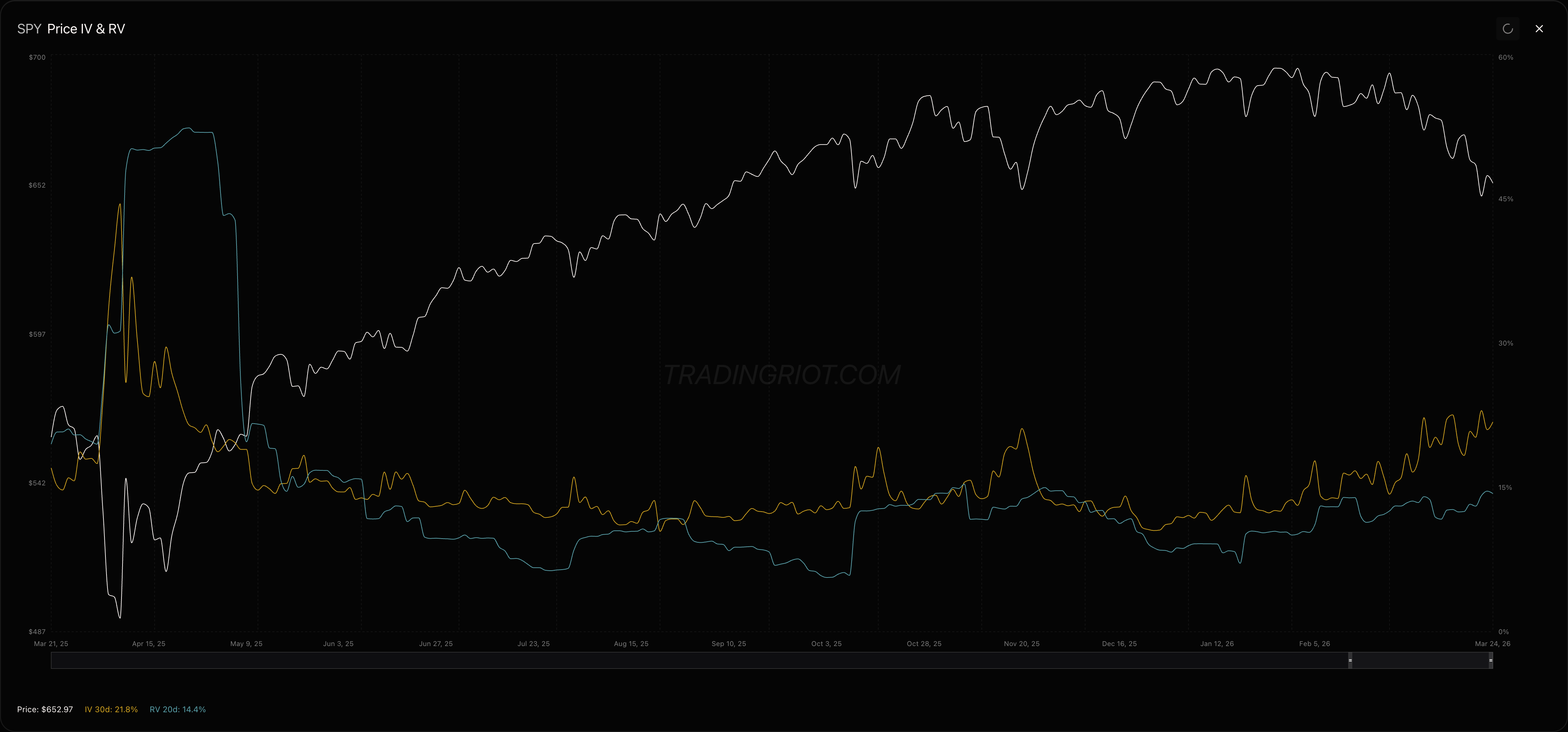
When IV is higher than RV, options are “expensive” relative to what actually materializes, and sellers have an edge. When IV is lower than RV, options are “cheap,” and buyers have an edge.

This sounds simple, but it’s the foundation of the entire variance risk premium, which is one of the most well-documented edges in options markets. We cover it extensively on TradingRiot.

Volatility Characteristics

Volatility has a few key properties that matter for trading.

First, it’s mean-reverting. Volatility tends to return to its long-term average. Extreme high vol eventually calms down. Extreme low vol eventually spikes. This is why selling vol at highs and buying at lows has an edge over time.

Second, it clusters. High-vol days tend to follow high-vol days. Quiet days tend to follow quiet days. Volatility comes in regimes, trending up or trending down before reverting. This means timing matters more than most people think.

Third, the relationship between price and volatility varies by asset class. In equities, there’s a strong negative correlation: vol rises when prices fall and drops when prices rise, this is the classic “staircase up, elevator down” effect, for most equities when prices go up, they go up slowly, but when they drop it tend to be very fast.

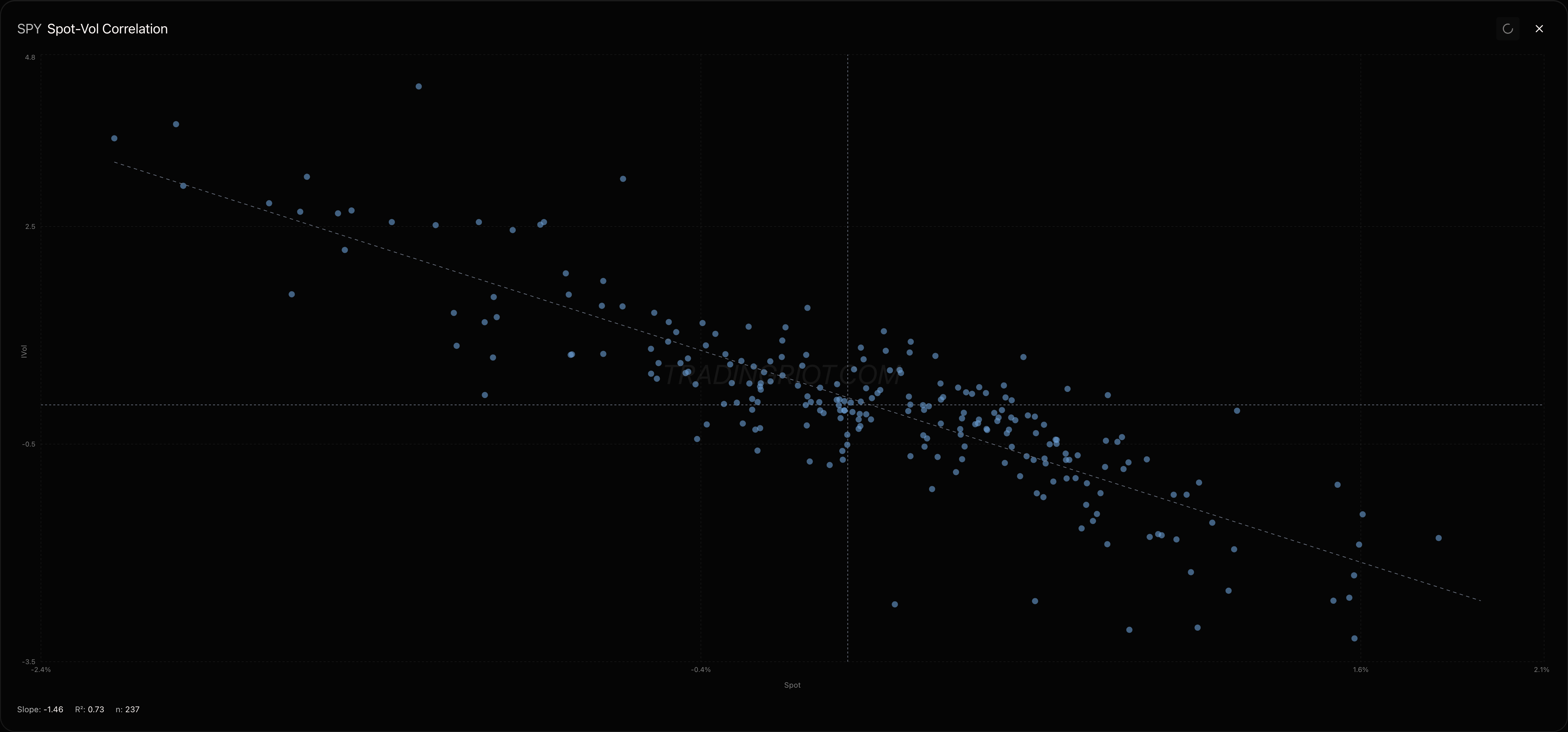
This creates the “cascade effect” and is the reason put skew exists in equity options.

Commodities behave differently. Some, like oil and grains, can have positive correlation where prices and vol rise together during supply shocks. Gold often has weak or mixed correlation. Crypto is generally negative like equities but weaker, and it can flip positive during euphoric rallies when vol expands alongside price. FX is mixed and depends on the specific pair and the broader risk-on/risk-off regime. Don’t assume equity vol behavior applies everywhere. Check the asset’s historical correlation.

Fourth, volatility has a term structure. Short-term IV often differs from long-term IV. Normally, longer-dated options have higher IV than shorter-dated ones. This is called contango. During crises, the term structure inverts: near-term IV spikes above long-term IV as the market panics about immediate risk. This is called backwardation or inversion.

IV Percentile and IV Rank

Raw IV numbers are hard to interpret without context. Is 30% IV high or low? It depends entirely on the stock. A 30% IV on a utility stock is extreme. A 30% IV on a meme stock is a quiet day. Percentile metrics provide context.

IV Percentile tells you what percentage of days in the past year had lower IV than the current level. If IV is at the 90th percentile, that means current IV is higher than 90% of all observations over the past year. It considers every data point, making it more robust.

IV Rank tells you where current IV sits relative to its 52-week range. The formula is (current IV - 52-week low) / (52-week high - 52-week low). It’s simpler but can be skewed by a single outlier spike that stretches the range.

High IV percentile (above 70%) generally favors premium selling. Low IV percentile (below 30%) generally favors premium buying. Our platform’s screeners surface these opportunities across over 1,000 markets.

That said, there are two common misconceptions worth addressing.

The first is “always sell when IV percentile is high.” Many strategies recommend selling options when IV percentile is above 50% or 70%. The problem is that high IV tends to cluster and persist longer than expected. If IV is at the 90th percentile, it often stays elevated for days or even months. Selling into rising vol can lead to significant losses as your short options gain value. It’s better to wait for signs of mean reversion, meaning IV that has started to decline from its peak, rather than selling just because it’s “high.”

The second is “low IV percentile means options are cheap, so it’s a good time to sell.” When IV percentile is very low (below 10-20%), premiums are small. Selling cheap options gives you poor risk-to-reward. You collect minimal premium but still face full downside risk. A vol spike from 15% to 30% can devastate short positions even if you correctly predicted the direction. Low IV environments are generally better for buying options or staying flat, not selling.

Term Structure

Implied volatility is not a single number. It varies across expirations, and this relationship is called the term structure.

As mentioned, in normal market conditions, longer-dated options have higher IV than shorter-dated ones. This makes intuitive sense. More time means more uncertainty, and more uncertainty means higher volatility priced in. This upward-sloping shape is called contango.

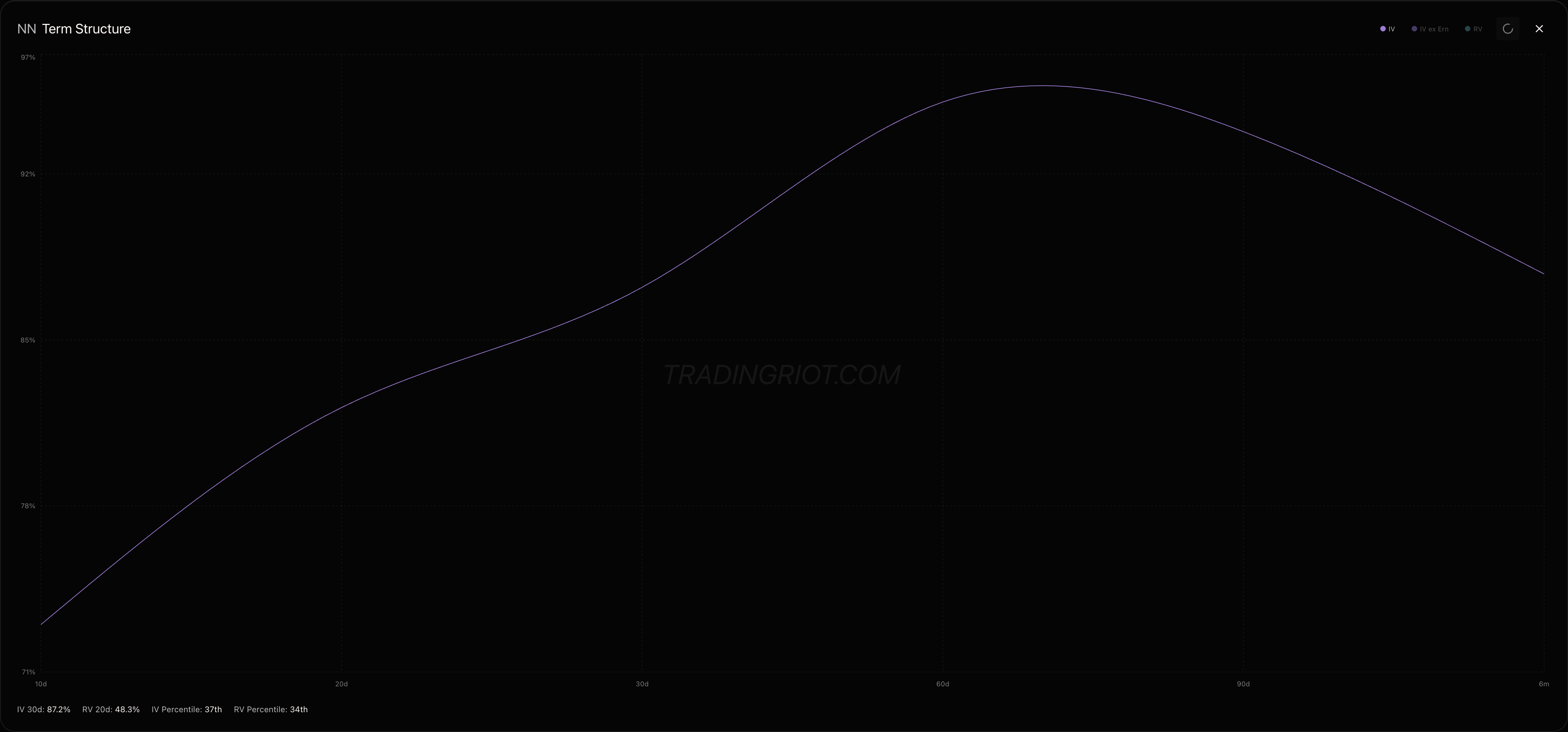
During crises, the term structure flips. Near-term IV spikes above long-term IV as the market panics about immediate risk while assuming things will eventually calm down. This is called backwardation or inversion.

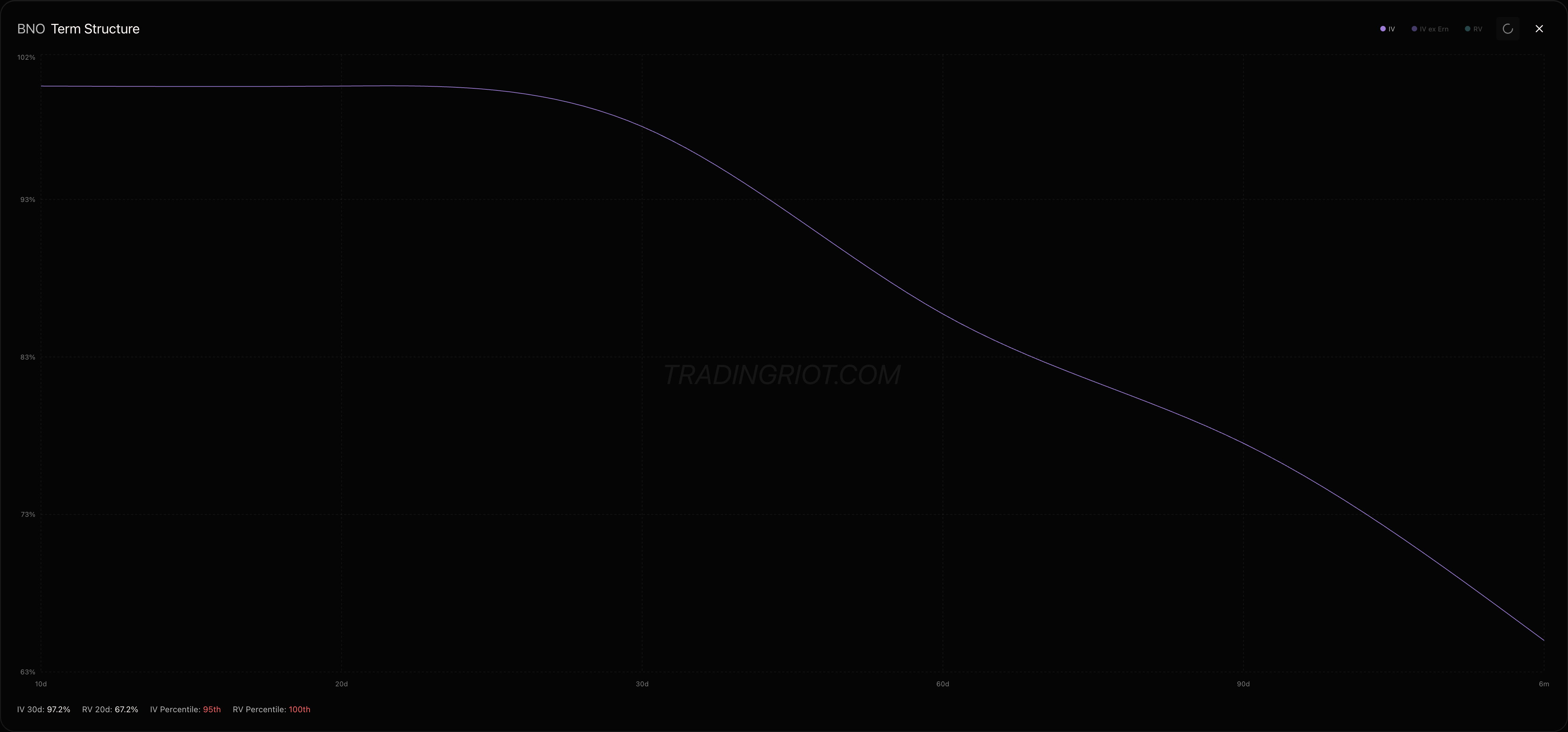
You can see this clearly in something like the VIX term structure. In a calm market, the VIX might sit at 15 with 3-month futures at 17 and 6-month futures at 19. That’s contango: calm and complacent. In a crisis, the VIX might spike to 35 while 3-month futures sit at 28 and 6-month futures at 24. That’s backwardation: fear and panic concentrated in the short term.

For example, as writing of this article, current conflict in Iran caused near-term VIX to be above the further expirations.

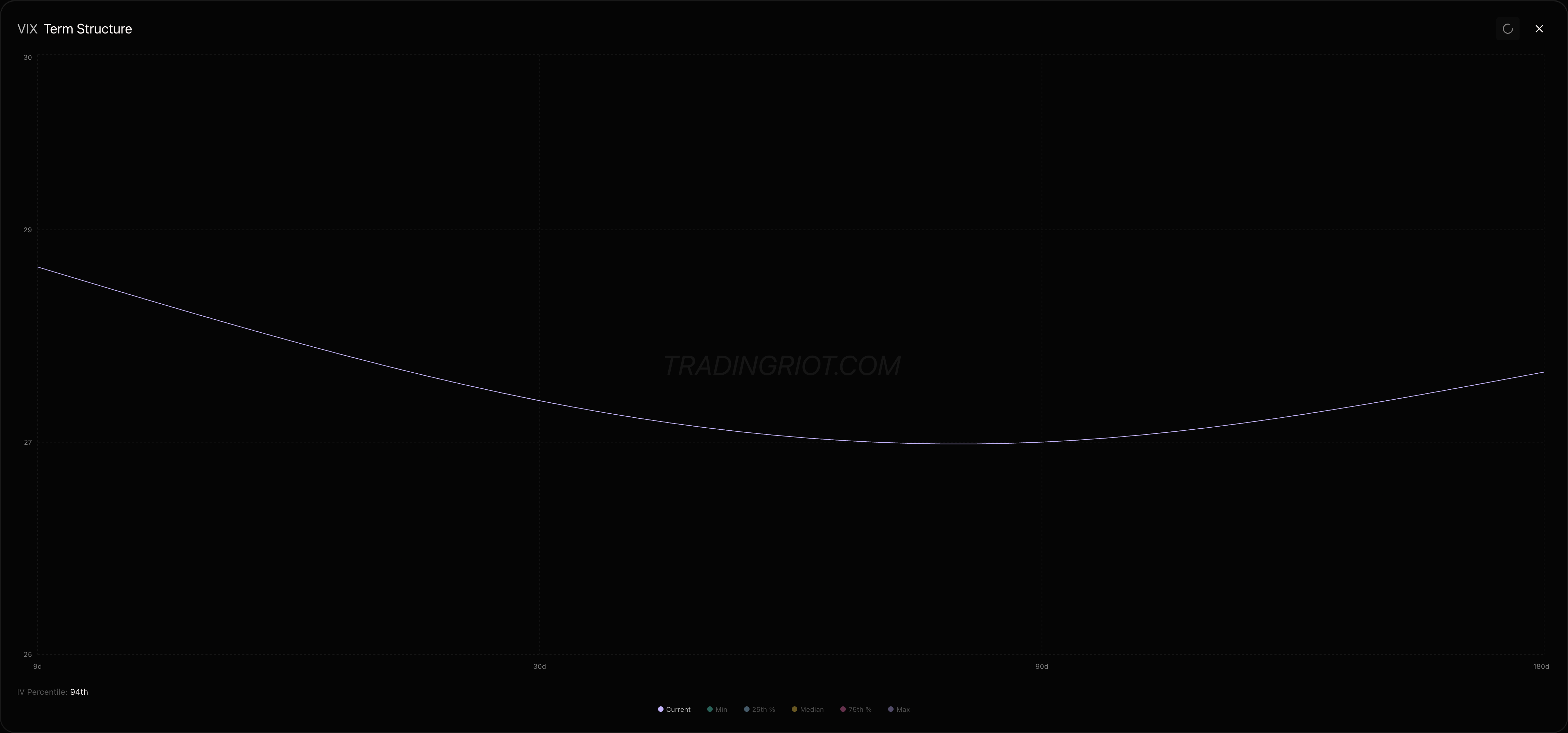
The shape of the term structure tells you a lot about market sentiment, and shifts between contango and backwardation often signal turning points worth paying attention to.

There’s also the concept of forward implied volatility, which lets you extract the vol the market is pricing for a specific future window by comparing two points on the term structure. It’s useful for calendar spreads, detecting events priced into specific windows, and comparing forward vol against historical realized vol for relative value trades. We’ll cover forward volatility in depth in a dedicated article.

Skew

If term structure describes how IV varies across expirations, skew describes how IV varies across strike prices for the same expiration.

In theory, Black-Scholes assumes all strikes should have the same IV. In reality, they never do. That deviation tells you about market expectations and positioning.

In equities, OTM puts typically have 3-8% higher IV than ATM options. OTM calls usually have slightly lower IV. This creates an asymmetric shape called the “smirk” rather than a symmetric smile.

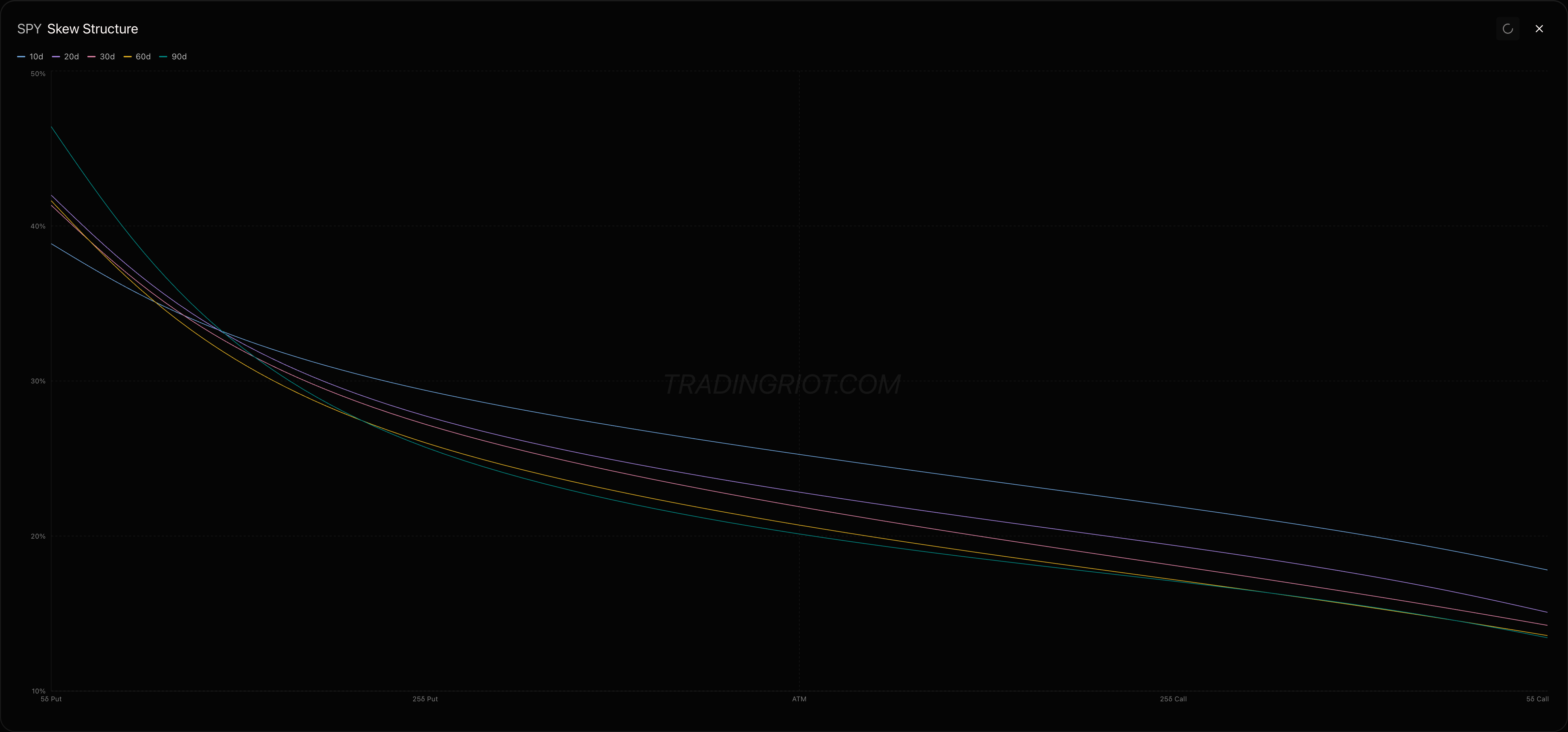
Skew also varies by expiration. Combine strike-axis skew with time-axis term structure and you get the volatility surface, a 3D representation of IV across all strikes and expirations. Short-dated options often have steeper skew with a more pronounced smirk. Longer-dated options have flatter skew as immediate crash fears fade.

Why Skew Exists

Skew is fundamentally a supply and demand imbalance. Options are priced by market makers who must hedge. When one side has more natural flow, prices adjust.

On the put side, there’s massive structural demand. Pension funds hedge equity portfolios because they’re mandated to. Insurance companies buy puts to meet regulatory requirements. Retail investors buy crash protection. Hedge funds buy tail hedges. On the other side, market makers sell these puts reluctantly and at premium prices, while some yield-seeking investors sell puts for income. More buyers than sellers means put prices get bid up, which shows up as higher IV for OTM puts.

On the call side, the dynamic reverses. Buyers are mostly speculators betting on rallies and retail traders buying lottery tickets. Sellers include a massive supply of covered call writers and market makers who are more willing to offer fair prices. More sellers than buyers means call prices stay lower, which means lower IV for OTM calls.

Beyond supply and demand, there are a few other forces that reinforce skew. The leverage effect plays a role: when stocks fall, company debt-to-equity rises, making equity riskier. This self-reinforcing cycle justifies higher put prices. There’s also asymmetric jump risk. Markets can gap down overnight in a crash, but they rarely gap up by the same magnitude. Puts need to price in that asymmetry. Finally, dealer hedging matters. Market makers who sell puts must buy stock as the price falls to stay delta-hedged. This buying pressure during crashes is limited by capital, so they charge more upfront, which means higher IV.

Measuring Skew

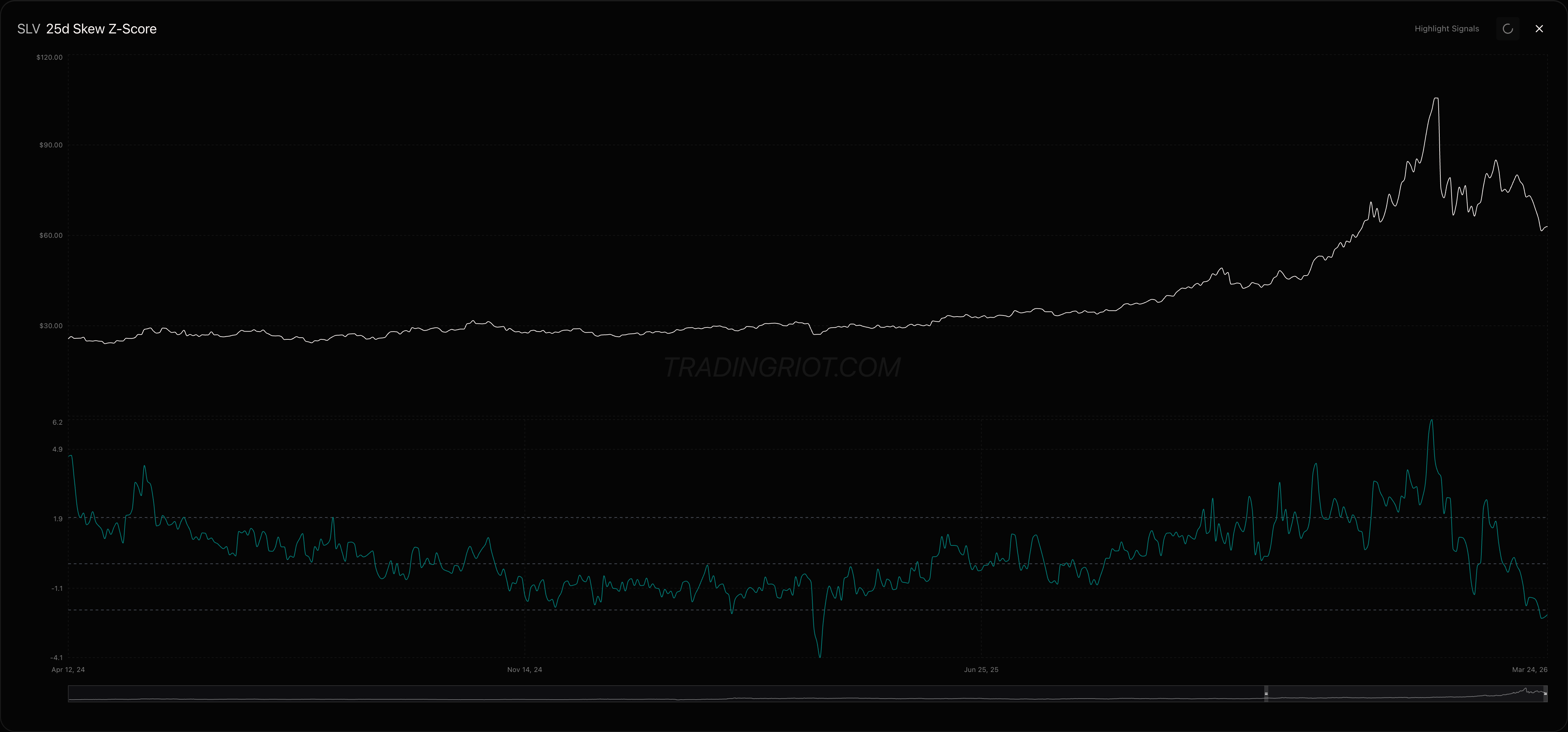
The most common way to measure skew is the 25-delta put-call skew, which is the difference between 25-delta put IV and 25-delta call IV.

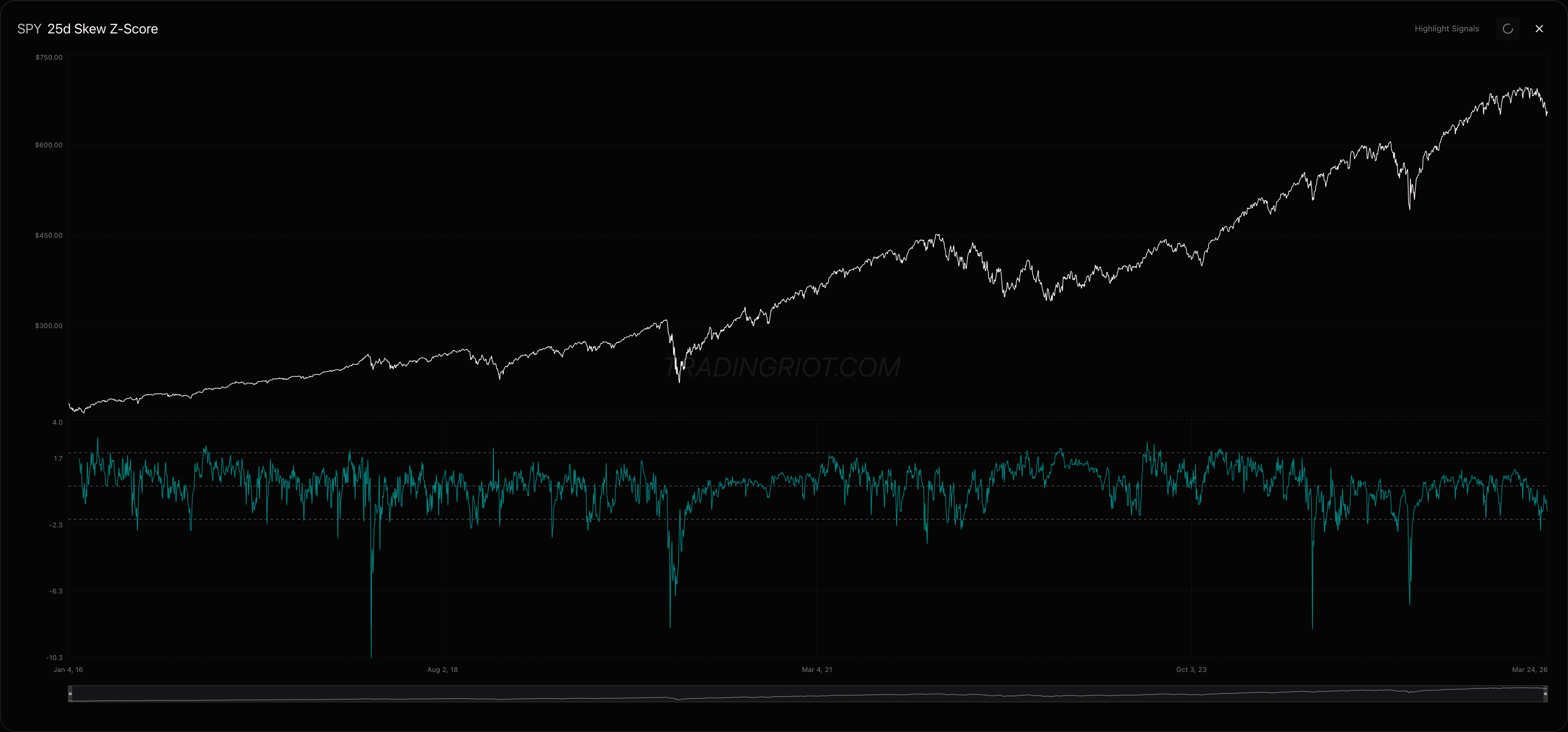
To make skew actionable, you can normalize it using a z-score, which compares current skew to its historical average. The chart above shows the SPY 25-delta skew z-score from our platform.

Negative z-scores mean puts are expensive relative to calls. You can see the sharp negative spikes lining up with selloffs in SPY, which makes sense. When the market drops, put demand surges and skew steepens. The more extreme the spike, the more panicked the demand for downside protection.

Positive z-scores mean calls are expensive relative to puts. This tends to happen during strong rallies or momentum-driven grinds higher, when upside speculation heats up and call demand pushes OTM call IV above its normal range.

A z-score beyond 2 or below -2 signals an extreme. Both can present opportunities. When skew is extremely negative and puts are expensive, there’s potential to sell put spreads and collect that elevated premium. When skew is flat or positive and puts are cheap, it might be a good time to buy protection before the market reprices risk.

Skew is not static. It shifts with market conditions. Sharp selloffs steepen skew as put demand surges. Rallies flatten skew as put demand fades. Slow grinds higher can sometimes push call skew into positive territory as momentum traders pile in.

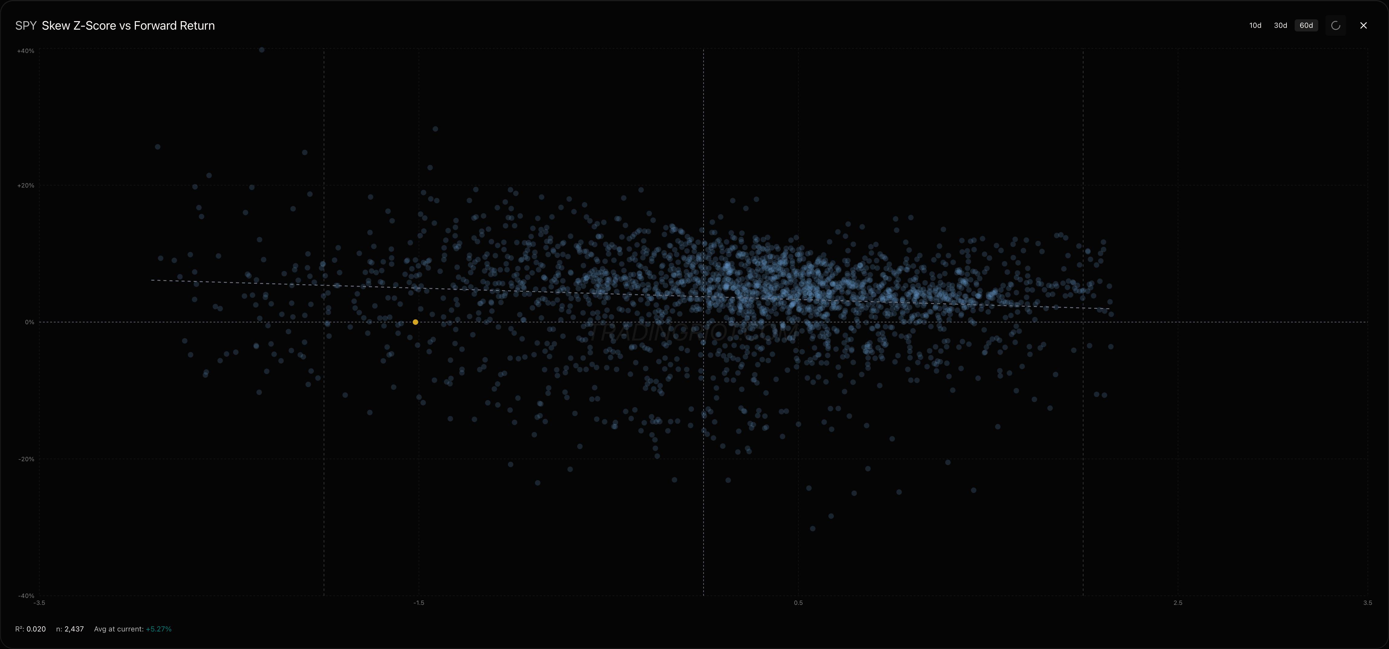
You can also use skew as a research input by plotting it against forward returns. The chart above shows SPY skew z-score on the x-axis against 60-day forward returns on the y-axis across 2,437 observations.

The R-squared is low at 0.020, which tells you skew alone is not a standalone predictor of direction. But look at the distribution. When skew is extremely negative (far left of the chart), forward returns tend to skew positive as the market bounces from panic. When skew is positive (right side), the spread of outcomes is more balanced. It's not a signal you trade blindly, but it adds context when combined with other factors like IV percentile and term structure. This scatter plot along with skew z-scores and term structure data are available for every stock and ETF on tradingriot.com.

Options Strategies

Now that you understand all of the important options dynamics, we can talk about strategies. Although these should be called payoff diagrams rather than strategies, since they are just structures you can use to speculate on prices.

As I already mentioned, when trading options, you will notice the lack of classic “Long” and “Short” buttons you might be used to from other derivatives. You trade calls and puts, and you can go both long and short on them.

When you are trading options, you can be either bullish or bearish, make a profit when markets are not moving, or profit on a significant move without being correct on the direction.

Let’s start with the simple things.

Single-Leg Trades

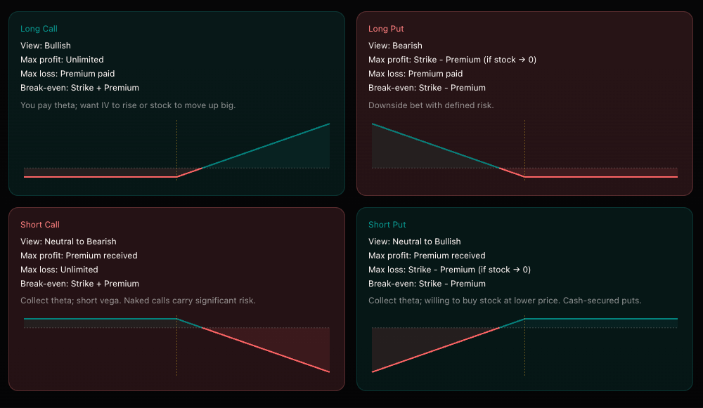
• When you buy a call, you are bullish. Your risk is the premium you paid, and your profit potential is unlimited when the market goes up.

• When you buy a put, you are bearish. Your risk is the premium you paid, and your profit potential is unlimited when the market goes down.

• When you sell a call, you are bearish. Your risk is unlimited, and your maximum gain is the premium you received.

• When you sell a put, you are bullish. Your risk is unlimited, and your maximum gain is the premium you received.

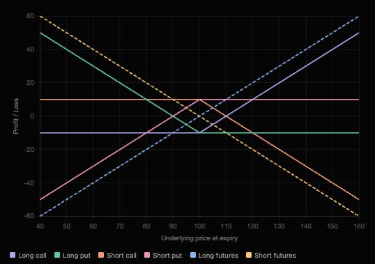
The chart above shows the payoff at expiration for all basic positions. The solid lines are options. The dashed lines are futures (buying and selling an ATM call and put at the same strike creates synthetic futures exposure with a linear payoff).

Notice the key difference. Futures payoffs are straight diagonal lines. You make or lose money linearly with every price move. Long futures profits when price goes up, short futures profits when price goes down. Simple.

Options payoffs have a kink. That kink is the strike price, and it’s what makes options fundamentally different from futures.

The long call (purple) loses only the premium paid if the price stays below the strike, then starts profiting once price moves above the strike plus the premium. Risk is capped, upside is not.

The long put (green) is the mirror image. It loses only the premium if price stays above the strike, then profits as price falls below the strike minus the premium.

The short call (orange) and short put (pink) are the exact opposite. They collect the premium upfront and keep it if price stays on the right side of the strike. But if price moves against them, losses grow with every tick. Capped reward, uncapped risk.

Compare the dashed futures lines to the solid options lines. Futures give you dollar-for-dollar exposure in both directions. Options let you choose your risk profile: pay a premium to cap your downside, or collect a premium and accept open-ended risk.

The thing about options is that you can buy or sell more of them simultaneously to create multi-leg positions.

There is a plethora of these “strategies” using multi-leg options. Some of them have insane names like jade lizard (who came up with that?). I personally think this is a little far-fetched, and instead of knowing all the different names, you should focus on understanding how the payouts on these work.

Vertical Spreads

The simplest multi-leg structure is a vertical spread. You buy one option and sell another at a different strike within the same expiration.

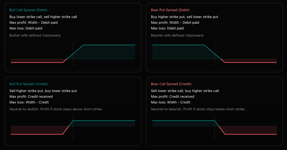
Debit spreads are the directional version. A bull call spread means you buy a lower strike call and sell a higher strike call against it. The short call partially finances your long call, reducing the premium you pay. The trade-off is that you cap your upside at the short strike. Bear put spreads work the same way in reverse: buy a higher strike put, sell a lower strike put.

Debit spreads are particularly useful when skew is extreme. If puts are expensive due to steep skew and you think the move has further to go, buying a put spread instead of a naked put drastically improves your risk-to-reward. You're selling the expensive wing back to the market and keeping the directional exposure. The same applies on the call side during momentum rallies when call skew gets bid up.

Credit spreads flip the logic. Instead of paying for a directional bet, you collect premium and profit if the market stays away from your short strike. A bull put spread means you sell a higher strike put and buy a lower strike put as protection. A bear call spread means you sell a lower strike call and buy a higher strike call above it.

Credit spreads typically have negative risk-to-reward. Your max loss is larger than your max profit. But the trade-off is that you don’t need the market to move in your favor. You just need it to stay relatively flat or not move against you past the short strike. Debit spreads are the opposite. They offer positive risk-to-reward but require momentum to continue in your direction to pay off.

Credit spreads work best in high IV environments where premiums are inflated. You collect more credit upfront, which gives you a wider breakeven and better probability of profit. The long option you buy defines your max loss, so unlike naked short options, your risk is capped on both sides.

Both debit and credit spreads define your max profit and max loss at entry. Max profit on a debit spread is the width between strikes minus the debit paid. Max loss is the debit. For credit spreads, max profit is the credit received. Max loss is the width between strikes minus the credit.

Ratio Spreads

Ratio spreads add an extra dimension. Instead of buying and selling the same number of contracts, you use uneven legs. The most common structure is a 1x2: buy one ATM or ITM option and sell two OTM options against it.

A 1x2 call ratio spread is for a moderately bullish view. You buy one call closer to the money and sell two further out. The extra short call finances the trade, often bringing it to a net credit. Max profit hits at the short strike where both short calls expire worthless and your long call has full value. The catch is that above the upper breakeven, you have a naked short call, so risk becomes unlimited to the upside.

The put ratio spread is the mirror image. Buy one put closer to the money, sell two further out. This one is particularly interesting in steep skew environments. You’re selling the expensive OTM puts that are inflated by skew demand and using them to finance your long put. If the market drops moderately to your short strike, you make maximum profit. If it crashes through the lower breakeven, the naked short put exposure kicks in and losses grow.

Ratio spreads are great for trading skew. When the options you’re selling have elevated IV relative to the ones you’re buying, you collect significantly more premium on the short legs, which widens your breakevens and can turn the entire structure into a net credit. You’re essentially monetizing the skew while still maintaining directional exposure.

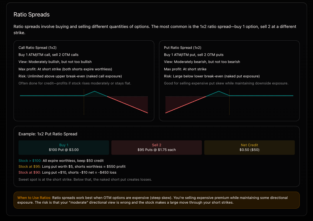
The important thing with ratio spreads is knowing when to get out. Since the naked leg creates technically unlimited risk if price blows through the short strike, managing the position and exiting at the right time is the difference between a clever trade and a disaster. But for traders who have a view on both direction and magnitude, they offer a payoff profile you can't replicate with simple verticals.

Risk Reversal

A risk reversal, also called a collar, combines a short option on one side with a long option on the other. The bullish version sells an OTM put and buys an OTM call. The bearish version buys an OTM put and sells an OTM call.

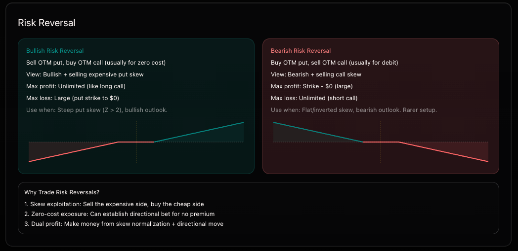
These are popular as hedging structures, but they’re also one of the best ways to trade skew. The idea is simple. When put skew is steep, OTM puts are expensive and OTM calls are relatively cheap. A bullish risk reversal lets you sell the expensive put and use that premium to finance the cheap call, often for zero cost or even a net credit.

Compare this to buying and selling an ATM call and put at the same strike, which creates synthetic futures exposure with a linear payoff. A risk reversal gives you similar directional exposure but benefits from the skew differential. You're getting paid for the asymmetry in implied volatility across strikes rather than paying fair value on both sides.

This makes risk reversals particularly effective when skew is elevated and you think the move is done. If the market just rallied hard and call skew spiked, selling that inflated cal premium and buying cheap put lets you position for a reversal while collecting the skew normalization as a bonus.

Taking such trade in SLV this year before the large sell-off was one of the most profitable structures to trade

You can profit from both the directional move and the skew compressing back to normal levels.

These are often my preferred structures for directional reversal trades. That said, you need to be careful. The short option leg carries unlimited loss potential. If you sell a put and the market keeps crashing through your strike, losses are substantial. Position sizing and exits matter just as much as the thesis.

Volatility Strategies

This is where options really separate themselves from every other instrument. The strategies above were all directional to some degree. You had a view on where the market was going. Volatility strategies don’t care about direction. They care about how much the market moves, or doesn’t.

The concept behind this is delta neutrality. When you buy both a call and a put at the same strike, the positive delta from the call and the negative delta from the put roughly cancel each other out. You’re not long or short the market. You’re long or short volatility itself.

Straddles and Strangles

A long straddle means buying an ATM call and an ATM put at the same strike. You profit if the market makes a big move in either direction. You don’t care which way, you just need it to move far enough to cover the premium you paid on both legs. Long straddles are long gamma, long vega, and short theta. You need realized volatility to exceed what implied volatility priced in. Every day that passes without a big move, theta eats into your position.

A long strangle is the cheaper version. Instead of buying ATM options, you buy OTM calls and OTM puts. The premium is lower, but the breakevens are wider. You need an even bigger move to profit.

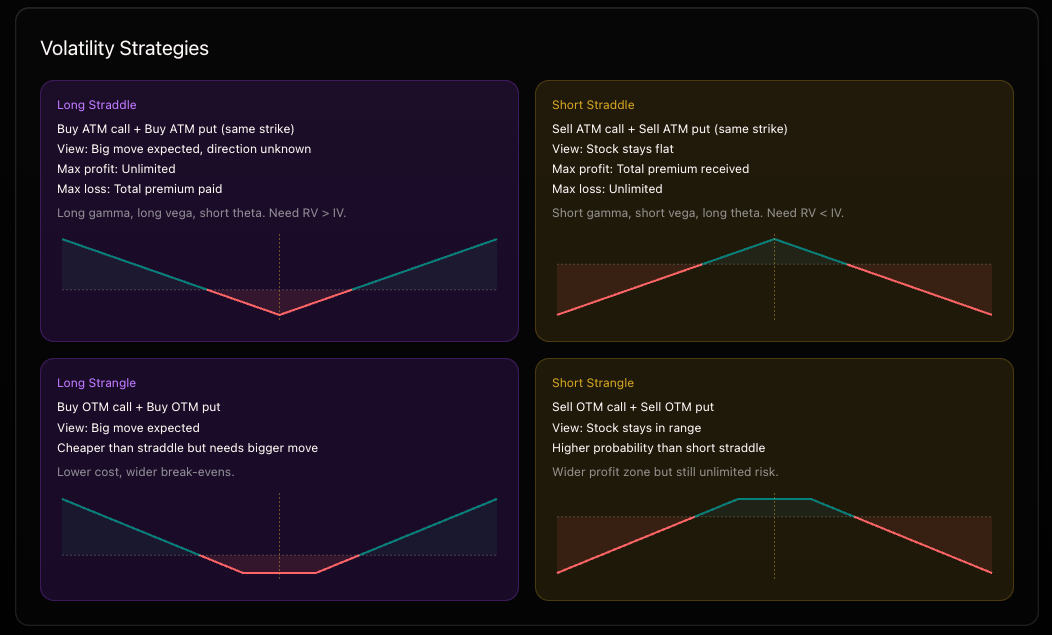
Flip both of these around and you get short straddles and short strangles. A short straddle means selling both the ATM call and ATM put. You collect the combined premium and profit if the market stays flat. You’re short gamma, short vega, and long theta. Time decay works in your favor, and you need implied volatility to overstate what actually happens. The risk is that a big move in either direction creates unlimited losses.

A short strangle sells OTM options on both sides instead of ATM. The profit zone is wider since the market has to move past either short strike before you start losing. Higher probability of profit, but still unlimited risk on both sides.

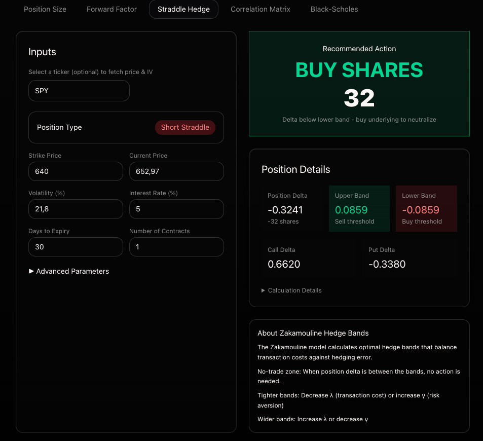
Delta Hedging

Here’s how it works. You sell an ATM straddle on SPY at the 657 strike. At entry, the position is roughly delta neutral. SPY then rallies to $662, and your short call gains delta while your short put loses it. Your position is now net short delta, meaning you’re losing money on the move up.

To neutralize this, you buy SPY shares (or futures) to offset the delta exposure. Now you’re delta neutral again. If SPY then drops back to $655, your position becomes net long delta from the shares you bought. You sell some shares to flatten out again.

Every time you rehedge, you’re locking in small losses. You bought shares higher and sold them lower. These rehedging costs are the realized volatility component of the trade. If the total cost of all your delta hedges (realized vol) is less than the premium you collected (implied vol), you profit. If the market whips around more than implied vol predicted, those hedging costs add up and you lose.

This is the core of volatility trading. You’re not betting on direction. You’re betting that the premium you collected overcompensates for the actual movement that materializes. The entire variance risk premium concept is built on this dynamic.

How often should you delta hedge? What delta should you actually hedge? Should you delta hedge at all or just take the loss on the chin?

These are all good questions. The main thing you need to think about is that delta hedging is trading. Trading costs money in spreads and commissions. Losing money on spreads and commissions sucks.

Because of that, you shouldn’t hedge sporadically but rather be strategic, setting delta bands where you hedge your delta back to zero. For any longer-term options, hedging more than once per day doesn’t make much sense.

You can use a free calculator on tradingriot.com that calculates hedging bands automatically for you, or you can just trade iron condors and butterflies with fixed loss.

Iron Condors and Iron Butterflies

If unlimited risk on short straddles and strangles makes you uncomfortable, iron condors and iron butterflies are the defined-risk versions.

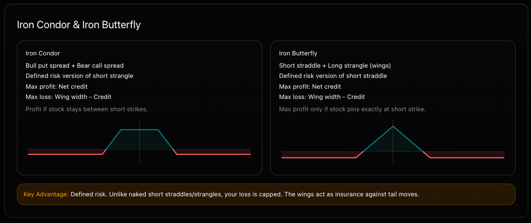
An iron condor is a bull put spread combined with a bear call spread. You sell options on both sides of the market and buy further OTM options as protection. Max profit is the net credit received, and you keep it if the market stays between your two short strikes. Max loss is the width of the wider wing minus the credit. It’s essentially a short strangle with wings that cap your risk.

An iron butterfly is the same idea but centered at one strike. You sell an ATM straddle and buy OTM options on both sides as protection. It’s a defined-risk version of the short straddle. Max profit is higher than an iron condor because ATM options collect more premium, but it only hits max profit if the stock pins exactly at the short strike. In practice, you’re usually taking it off before expiration once you’ve captured enough of the decay.

The key advantage of both structures is that the wings act as insurance against tail moves. Unlike naked short straddles and strangles, you know your worst-case loss at entry.

When buying wings for protection, I see people often trying to get comfortable and create a good risk-to-reward ratio. This is the wrong approach. Spending too much on wings eats a lot of your premium, and it doesn’t really make sense.

When buying wings, you should only do it for the catastrophic case of the underlying teleporting overnight, the kind of move that would send you two tax brackets lower automatically.

I often go for 1-10 delta wings and try not to spend more than 5% of the credit I’m receiving.

To end this chapter, here is return profile per structure (I left out calendar spreads since they tie to forward volatility that I decided to not cover in this article).

Conclusion

Was I able to cover everything you need to know about options trading?

I hope so, but I have likely missed something. At the end of the day, there are whole books written about this stuff. Option Volatility and Pricing by Sheldon Natenberg or Options, Futures, and Other Derivatives by John Hull naturally come to mind.

That being said, I think this gives you a very solid primer to understand options. In the next articles, I will dive deeper into different trading strategies using options.